#' ---	
#' title: "DSPA2: Data Science and Predictive Analytics (UMich HS650)"	
#' subtitle: "<h2><u>Chapter 1: Introduction</u></h2>"	
#' author: "<h3>SOCR/MIDAS (Ivo Dinov)</h3>"	
#' date: "`r format(Sys.time(), '%B %Y')`"	
#' tags: [DSPA, SOCR, MIDAS, Big Data, Predictive Analytics] 	
#' output:	
#'   html_document:	
#'     theme: spacelab	
#'     highlight: tango	
#'     includes:	
#'       before_body: SOCR_header.html	
#'     toc: true	
#'     number_sections: true	
#'     toc_depth: 2	
#'     toc_float:	
#'       collapsed: false	
#'       smooth_scroll: true	
#'     code_folding: show	
#'     self_contained: yes	
#' ---	
#' 	
#' We start the DSPA journey with an overview of the mission and objectives of this textbook. Some early examples of driving motivational problems and challenges provide context into the common characteristics of big (biomedical and health) data. We will define data science and predictive analytics and emphasize the importance of their ethical, responsible, and reproducible practical use. This chapter also covers the foundations of R, contrasts R against other languages and computational data science platforms and introduces basic functions and data objects, formats, and simulation.	
#' 	
#' # Motivation	
#' 	
#' Let's start with a quick overview illustrating some common data science challenges, qualitative descriptions of the fundamental principles, and awareness about the power and potential pitfalls of modern data-driven scientific inquiry.	
#' 	
#' ## DSPA Mission and Objectives	
#' 	
#' The second edition of this textbook ([DSPA2](https://dspa2.predictive.space))is based on the [HS650: Data Science and Predictive Analytics (DSPA) course](https://predictive.space/) I teach at the University of Michigan and the [first DSPA edition](https://dspa.predictive.space/). These materials collectively aim to provide learners with a deep understanding of the challenges, appreciation of the enormous opportunities, and a solid methodological foundation for designing, collecting, managing, processing, interrogating, analyzing and interpreting complex health and biomedical data. Readers that finish this course of training and successfully complete the examples and assignments included in the book will gain unique skills and acquire a tool-chest of methods, software tools, and protocols that can be applied to a broad spectrum of Big Data problems.	
#' 	
#'  - **Vision**: Enable active-learning by integrating driving motivational challenges with mathematical foundations, computational statistics, and modern scientific inference	
#'  - **Values**: Effective, reliable, reproducible, and transformative data-driven discovery supporting open-science	
#'  - **Strategic priorities**: Trainees will develop scientific intuition, computational skills, and data-wrangling abilities to tackle Big biomedical and health data problems. Instructors will provide well-documented R-scripts and software recipes implementing atomic data-filters as well as complex end-to-end predictive big data analytics solutions.	
#' 	
#' Before diving into the mathematical algorithms, statistical computing methods, software tools, and health analytics covered in the remaining chapters, we will discuss several *driving motivational problems*. These will ground all the subsequent scientific discussions, data modeling, and computational approaches.	
#' 	
#' ## Examples of driving motivational problems and challenges	
#' 	
#' For each of the studies below, we illustrate several clinically-relevant scientific questions, identify appropriate data sources, describe the types of data elements, and pinpoint various complexity challenges.	
#' 	
#' ### Alzheimer's Disease 	
#' 	
#'  -	Identify the relation between observed clinical phenotypes and expected behavior;	
#'  -	Prognosticate future cognitive decline (3-12 months prospectively) as a function of imaging data and clinical assessment (both model-based and model-free machine learning prediction methods will be used);	
#'  -	Derive and interpret the classifications of subjects into clusters using the harmonized and aggregated data from multiple sources.	
#' 	
#' Data Source |           Sample Size/Data Type    |   Summary       	
#' ------------|------------------------------------|-----------------	
#' [ADNI Archive](https://www.adni-info.org) | Clinical data: demographics, clinical assessments, cognitive assessments; Imaging data: sMRI, fMRI, DTI, PiB/FDG PET; Genetics data: Ilumina SNP genotyping; Chemical biomarker: lab tests, proteomics. Each data modality comes with a different number of cohorts. Generally, $200\le N \le 1200$. For instance, previously conducted ADNI studies with N>500 [ [doi: 10.3233/JAD-150335](https://www.ncbi.nlm.nih.gov/pubmed/26444770), [doi: 10.1111/jon.12252](https://www.ncbi.nlm.nih.gov/pubmed/25940587), [doi: 10.3389/fninf.2014.00041](https://www.ncbi.nlm.nih.gov/pubmed/24795619)] | ADNI provides interesting data modalities, multiple cohorts (e.g., early-onset, mild, and severe dementia, controls) that allow effective model training and validation [NACC Archive](https://www.alz.washington.edu) | Clinical data: treatments, diagnosis, clinical assessments, cognitive tests; Imaging data: sMRI, fMRI; Genetics data: SNP genotypes; Biospecimen: blood, buffy coat, brain tissue; Demographics: family history, phenotypes. This collection includes over 5,000 unique subjects with an average of 6 years of follow-up. Not all data elements/cases are complete | NACC data facilitates the exploration of GWAS and diverse phenotypes. These data provide means to do exploratory neuropathological studies of dementia and cognitive decline, accounting for risk alleles like APOE $\epsilon 4$ and protective alleles APOE $\epsilon 2$	
#' 	
#' ### Parkinson's Disease 	
#' 	
#'  - Predict the clinical diagnosis of patients using all available data (with and without the UPDRS clinical assessment, which is the basis of the clinical diagnosis by a physician);	
#'  - Compute derived neuroimaging and genetics biomarkers that can be used to model the disease progression and provide automated clinical decisions support;	
#'  - Generate decision trees for numeric and categorical responses (representing clinically relevant outcome variables) that can be used to suggest an appropriate course of treatment for specific clinical phenotypes.	
#' 	
#' Data Source |           Sample Size/Data Type    |   Summary       	
#' ------------|------------------------------------|-----------------	
#' [PPMI Archive](https://www.ppmi-info.org) | Demographics: age, medical history, sex; Clinical data: physical, verbal learning and language, neurological and olfactory (University of Pennsylvania Smell Identification Test, UPSIT) tests), vital signs, MDS-UPDRS scores (Movement Disorder; Society-Unified Parkinson's Disease Rating Scale), ADL (activities of daily living), Montreal Cognitive Assessment (MoCA), Geriatric Depression Scale (GDS-15); Imaging data: structural MRI; Genetics data: llumina ImmunoChip (196,524 variants) and NeuroX (covering 240,000 exonic variants) with 100% sample success rate, and 98.7% genotype success rate genotyped for APOE e2/e3/e4. Three cohorts of subjects; Group 1 = {de novo PD Subjects with a diagnosis of PD for two years or less who are not taking PD medications}, N1 = 263; Group 2 = {PD Subjects with Scans without Evidence of a Dopaminergic Deficit (SWEDD)}, N2 = 40; Group 3 = {Control Subjects without PD who are 30 years or older and who do not have a first degree blood relative with PD}, N3 = 127 | The longitudinal PPMI dataset including clinical, biological and imaging data (screening, baseline, 12, 24, and 48 month follow-ups) may be used conduct model-based predictions as well as model-free classification and forecasting analyses	
#' 	
#' ### Drug and substance use 	
#' 	
#'  - Is the Risk for Alcohol Withdrawal Syndrome (RAWS) screen a valid and reliable tool for predicting alcohol withdrawal in an adult medical inpatient population?	
#'  - What is the optimal cut-off score from the AUDIT-C to predict alcohol withdrawal based on RAWS screening?	
#'  - Should any items be deleted from, or added to, the RAWS screening tool to enhance its performance in predicting the emergence of alcohol withdrawal syndrome in an adult medical inpatient population?	
#' 	
#' Data Source |           Sample Size/Data Type    |   Summary       	
#' ------------|------------------------------------|-----------------	
#' MAWS Data / UMHS EHR / [WHO AWS Data](https://apps.who.int/gho/data/node.main-amro.A1311?lang=en)	| Scores from Alcohol Use Disorders Identification Test-Consumption (AUDIT-C) [49], including dichotomous variables for any current alcohol use (AUDIT-C, question 1), total AUDIT-C score > 8, and any positive history of alcohol withdrawal syndrome (HAWS) | ~1,000 positive cases per year among 10,000 adult medical inpatients, % RAWS screens completed, % positive screens, % entered into MAWS protocol who receive pharmacological treatment for AWS, % entered into MAWS protocol without a completed RAWS screen | Blood alcohol level (BAL) on admission, urine drug screen, mean corpuscular volume (MCV), liver enzymes (ALT, AST, CDT, GGTP), cigarette use, other tobacco and/or nicotine use, including e-cigarettes, comorbid medical, psychiatric, and/or other substance use diagnoses	
#'  	
#' 	
#' ### Amyotrophic lateral sclerosis  	
#' 	
#' * Identify the most highly-significant variables that have power to jointly predict the progression of ALS (in terms of clinical outcomes like [ALSFRS](http://www.outcomes-umassmed.org/ALS/sf12.aspx) and muscle function)	
#' * Provide a decision tree prediction of adverse events based on subject phenotype and 0-3 month clinical assessment changes	
#' 	
#' Data Source |           Sample Size/Data Type    |   Summary       	
#' ------------|------------------------------------|-----------------	
#' [ProAct Archive](http://www.ALSdatabase.org) | Over 100 clinical variables are recorded for all subjects including: Demographics: age, race, medical history, sex; Clinical data:  Amyotrophic Lateral Sclerosis Functional Rating Scale (ALSFRS), adverse events, onset_delta, onset_site, drugs use (riluzole)	The PRO-ACT training dataset contains clinical and lab test information of 8,635 patients. Information of 2,424 study subjects with valid gold standard ALSFRS slopes will be used in out processing, modeling and analysis | The time points for all longitudinally varying data elements will be aggregated into signature vectors. This will facilitate the modeling and prediction of ALSFRS slope changes over the first three months (baseline to month 3)	
#' 	
#' ### Normal Brain Visualization	
#' 	
#' The [SOCR Brain Visualization App](https://socr.umich.edu/HTML5/BrainViewer) has preloaded sMRI, ROI labels, and fiber track models for a normal brain. It also allows users to drag-and-drop their data into the browser to visualize and navigate through the stereotactic data (including imaging, parcellations and tractography).	
#' 	
#' ![](http://socr.umich.edu/Udall_PD/images/UdallPD_Carousel_01.png)	
#' ![](http://socr.umich.edu/Udall_PD/images/UdallPD_Carousel_02.png)	
#' 	
#' ### Neurodegeneration	
#' 	
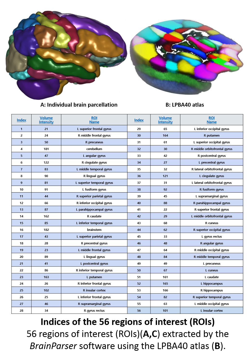
#' A recent study of [Structural Neuroimaging in Alzheimer's Disease](https://www.ncbi.nlm.nih.gov/pubmed/26444770) illustrates the Big Data challenges in modeling complex neuroscientific data. Specifically, 808 [ADNI](https://adni.loni.usc.edu/) subjects were divided into 3 groups: 200 subjects with Alzheimer's disease (AD), 383 subjects with mild cognitive impairment (MCI), and 225 asymptomatic normal controls (NC). Their sMRI data were parcellated using [BrainParser](https://www.loni.usc.edu/Software/BrainParser), and the 80 most important neuroimaging biomarkers were extracted using the global shape analysis Pipeline workflow. Using a pipeline implementation of Plink, the authors obtained 80 SNPs highly-associated with the imaging biomarkers. The authors observed significant correlations between genetic and neuroimaging phenotypes in the 808 ADNI subjects. These results suggest that differences between AD, MCI, and NC cohorts may be examined by using powerful joint models of morphometric, imaging and genotypic data. 	
#' 	
#' ![](http://www.socr.umich.edu/people/dinov/2017/Spring/DSPA_HS650/images/AD_Moon_Dinov_2016_F1.png)	
#' 	
#' ### Genomics computing	
#' 	
#' #### Genetic Forensics - 2013-2016 Ebola Outbreak	
#' 	
#' This [HHMI disease detective activity](https://www.hhmi.org/biointeractive/ebola-disease-detectives) illustrates genetic analysis of sequences of Ebola viruses isolated from patients in Sierra Leone during the Ebola outbreak of 2013-2016. Scientists track the spread of the virus using the fact that most of the genome is identical among individuals of the same species, most similar for genetically related individuals, and more different as the hereditary distance increases. DNA profiling capitalizes on these genetic differences. In particular, in regions of noncoding DNA, which is DNA that is not transcribed and translated into a protein. Variations in noncoding regions impact less individual's traits. Such changes in noncoding regions may be immune to natural selection.  DNA variations called **short tandem repeats (STRs)** are short bases, typically 2-5 bases long, that repeat multiple times. The repeat units are found at different locations, or loci, throughout the genome. Every STR has multiple alleles. These allele variants are defined by the **number of repeat units** present or by the **length of the repeat sequence**. STR are surrounded by non-variable segments of DNA known as flanking regions. The STR allele in the Figure below could be denoted by "6", as the repeat unit (GATA) repeats 6 times, or as 70 base pairs (bps) because its length is 70 bases in length, including the starting/ending flanking regions. Different alleles of the same STR may correspond to different numbers of GATA repeats, with the same flanking regions.	
#' 	
#' <div style="width:65%; margin:0 auto;">	
#' ![](http://www.socr.umich.edu/people/dinov/2017/Spring/DSPA_HS650/images/HHMI_BioInteractive_Ebola.png)	
#' </div>	
#' 	
#' #### Next Generation Sequence (NGS) Analysis	
#' 	
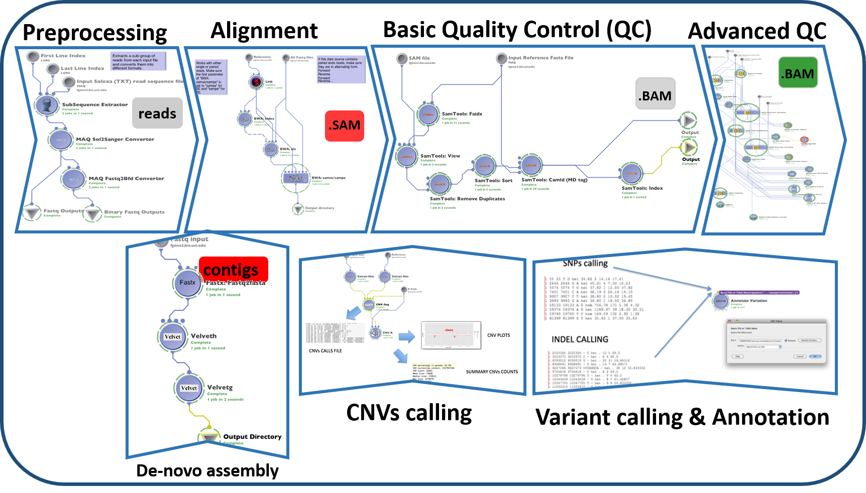
#' Whole-genome and exome sequencing include essential clues for identifying genes responsible for simple Mendelian inherited disorders. This [paper proposed methods can be applied to complex disorders based on population genetics](http://www.mdpi.com/2073-4425/3/3/545). Next generation sequencing (NGS) technologies include bioinformatics resources to analyze the dense and complex sequence data. The Graphical Pipeline for Computational Genomics (GPCG) performs the computational steps required to analyze NGS data. The GPCG implements flexible workflows for basic sequence alignment, sequence data quality control, single nucleotide polymorphism analysis, copy number variant identification, annotation, and visualization of results. Applications of NGS analysis provide clinical utility for identifying miRNA signatures in diseases. Enabling hypotheses testing about the functional role of variants in the human genome will help to pinpoint the genetic risk factors of many diseases (e.g., neuropsychiatric disorders).	
#' 	
#' ![](http://www.socr.umich.edu/people/dinov/2017/Spring/DSPA_HS650/images/GPCG_Torri_Dinov.png)  	
#' 	
#' #### Neuroimaging-genetics 	
#' 	
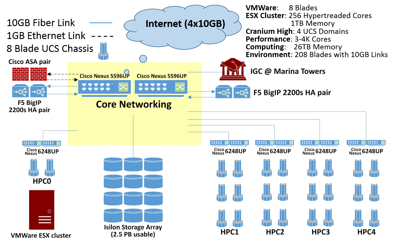
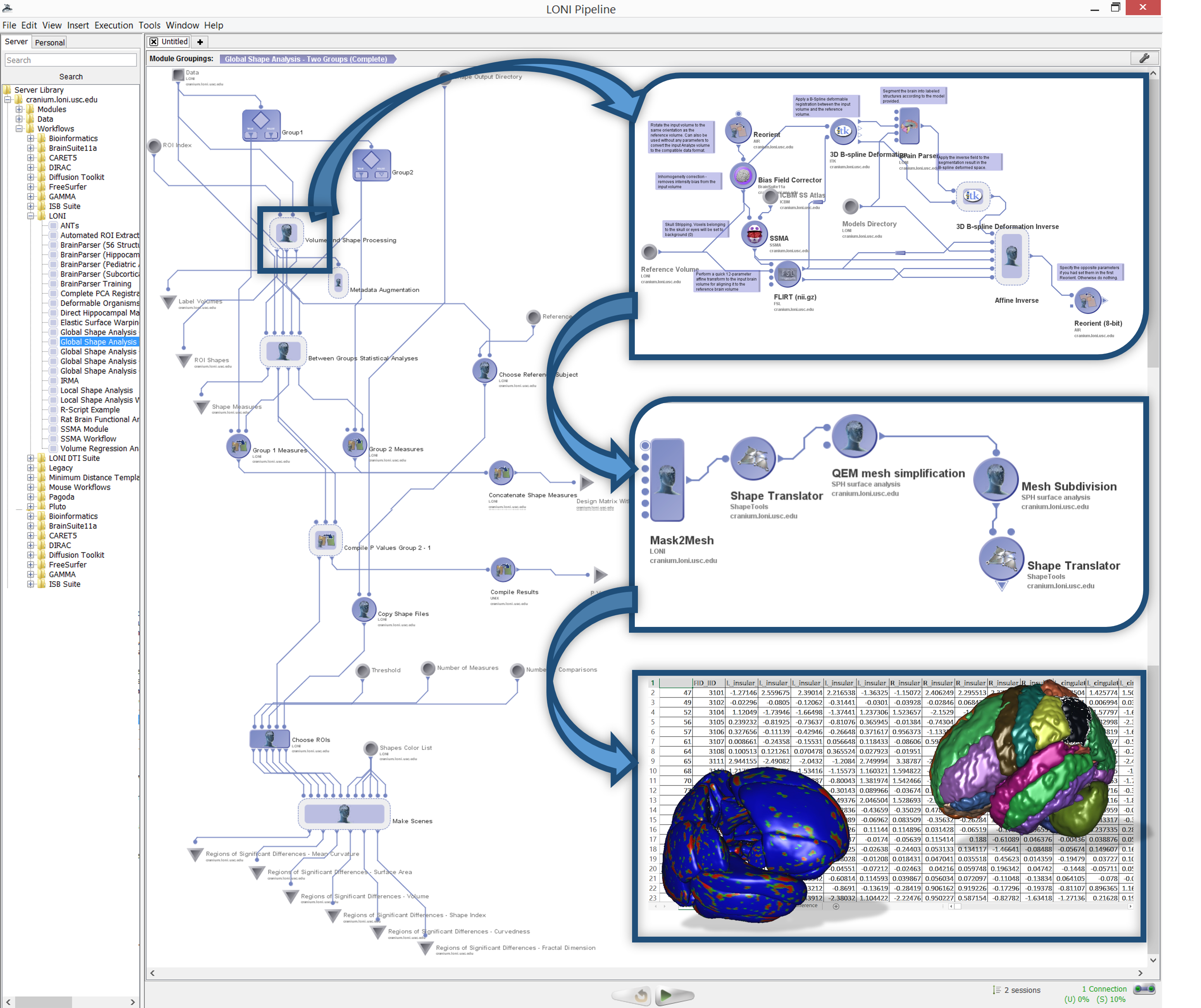
#' A [computational infrastructure for high-throughput neuroimaging-genetics (doi: 10.3389/fninf.2014.00041)](http://journal.frontiersin.org/article/10.3389/fninf.2014.00041/full) facilitates the data aggregation, harmonization, processing and interpretation of multisource imaging, genetics, clinical and cognitive data. A unique feature of this architecture is the graphical user interface to the Pipeline environment. Through its client-server architecture, the Pipeline environment provides a graphical user interface for designing, executing, monitoring, validating, and disseminating complex protocols that utilize diverse suites of software tools and web-services. These pipeline workflows are represented as portable XML objects, which transfer the execution instructions and user specifications from the client user machine to remote pipeline servers for distributed computing. Using Alzheimer's and Parkinson's data, this study provides examples of translational applications using this infrastructure	
#' 	
#' ![](http://www.socr.umich.edu/people/dinov/2017/Spring/DSPA_HS650/images/LONI_Cranium_2014.png)	
#' 	
#' ## Common Characteristics of *Big (Biomedical and Health) Data* 	
#' 	
#' Software developments, student training, utilization of Cloud or IoT service platforms, and methodological advances associated with Big Data Discovery Science all present existing opportunities for learners, educators, researchers, practitioners and policy makers, alike. A review of many biomedical, health informatics and clinical studies suggests that there are indeed common characteristics of complex big data challenges. For instance, imagine analyzing observational data of thousands of Parkinson's disease patients based on tens-of-thousands of signature biomarkers derived from multi-source imaging, genetics, clinical, physiologic, phenomics and demographic data elements. IBM had defined the qualitative characteristics of Big Data as 4V's: **Volume, Variety, Velocity** and **Veracity** (there are additional V-qualifiers that can be added).	
#' 	
#' More recently ([PMID:26998309](https://www.ncbi.nlm.nih.gov/pubmed/26998309)) we defined a constructive characterization of Big Data that clearly identifies the methodological gaps and necessary tools:	
#' 	
#' BD Dimensions | Tools	
#' --------------|-------	
#' Size | Harvesting and management of vast amounts of data	
#' Complexity | Wranglers for dealing with heterogeneous data	
#' Incongruency | Tools for data harmonization and aggregation	
#' Multi-source | Transfer and joint modeling of disparate elements	
#' Multi-scale | Macro to meso to micro scale observations 	
#' Time | Techniques accounting for longitudinal patterns in the data	
#' Incomplete | Reliable management of missing data	
#' 	
#' ## Data Science	
#' 	
#' *Data science* is an emerging new field that (1) is extremely transdisciplinary - bridging between the theoretical, computational, experimental, and biosocial areas, (2) deals with enormous amounts of complex, incongruent and dynamic data from multiple sources, and (3) aims to develop algorithms, methods, tools and services capable of ingesting such datasets and generating semi-automated decision support systems. The latter can mine the data for patterns or motifs, predict expected outcomes, suggest clustering or labeling of retrospective or prospective observations, compute data signatures or fingerprints, extract valuable information, and offer evidence-based actionable knowledge. Data science techniques often involve data manipulation (wrangling), data harmonization and aggregation, exploratory or confirmatory data analyses, predictive analytics, validation and fine-tuning. 	
#' 	
#' ## Predictive Analytics	
#' 	
#' *Predictive analytics* is the process of utilizing advanced mathematical formulations, powerful statistical computing algorithms, efficient software tools and services to represent, interrogate and interpret complex data. As its name suggests, a core aim of predictive analytics is to forecast trends, predict patterns in the data, or prognosticate the process behavior either within the range or outside the range of the observed data (e.g., in the future, or at locations where data may not be available). In this context, *process* refers to a natural phenomenon that is being investigated by examining proxy data. Presumably, by collecting and exploring the intrinsic data characteristics, we can track the behavior and unravel the underlying mechanism of the system.	
#' 	
#' The fundamental goal of predictive analytics is to identify relationships, associations, arrangements or motifs in the dataset, in terms of space, time, features (variables) that may reduce the dimensionality of the data, i.e., its complexity. Using these process characteristics, predictive analytics may predict unknown outcomes, produce estimations of likelihoods or parameters, generate classification labels, or contribute other aggregate or individualized forecasts. We will discuss how the outcomes of these predictive analytics can be refined, assessed and compared, e.g., between alternative methods. The underlying assumptions of the specific predictive analytics technique determine its usability, affect the expected accuracy, and guide the (human) actions resulting from the (machine) forecasts. In this textbook, we will discuss supervised and unsupervised, model-based and model-free, classification and regression, as well as deterministic, stochastic, classical and machine learning-based techniques for predictive analytics. The type of the expected outcome (e.g., binary, polytomous, probability, scalar, vector, tensor, etc.) determines if the predictive analytics strategy provides prediction, forecasting, labeling, likelihoods, grouping or motifs.	
#' 	
#' ## High-throughput Big Data Analytics	
#' 	
#' The [Pipeline Environment](https://pipeline.loni.usc.edu) provides a large tool chest of software and services that can be integrated, merged and processed. The [Pipeline workflow library](https://pipeline.loni.usc.edu/explore/library-navigator/) and the [workflow miner](https://pipeline.loni.usc.edu/products-services/workflow-miner/) illustrate much of the functionality that is available. A [Java-based](https://pipeline.loni.usc.edu/products-services/pws/) and an [HTML5 webapp based](https://pipeline.loni.usc.edu/products-services/webapp/) graphical user interfaces provide access to a powerful 4,000 core grid compute server.	
#' 	
#' ![](http://www.socr.umich.edu/people/dinov/2017/Spring/DSPA_HS650/images/PPMI_BDDS_GSA_PipeProtocol.png)	
#' 	
#' ## Examples of data repositories, archives and services	
#' 	
#' There are many sources of data available on the Internet. A number of them provide open-access to the data based on FAIR (Findable, Accessible, Interoperable, Reusable) principles. Below are examples of open-access data sources that can be used to test the techniques presented in the textbook. We demonstrate the tasks of retrieval, manipulation, processing, analytics and visualization using example datasets from these archives.	
#' 	
#'  - [SOCR Wiki Data](https://wiki.socr.umich.edu/index.php/SOCR_Data)	
#'  - [SOCR Canvas datasets](https://umich.instructure.com/courses/38100/files/folder/data)	
#'  - [SOCR Case-Studies](https://umich.instructure.com/courses/38100/files/folder/Case_Studies)	
#'  - [XNAT](https://central.xnat.org/)	
#'  - [IDA](https://ida.loni.usc.edu/)	
#'  - [NIH dbGaP](https://dbgap.ncbi.nlm.nih.gov/)	
#'  - [Data.gov](https://data.gov/)	
#' 	
#' ## Responsible Data Science and Ethical Predictive Analytics	
#' 	
#' In addition to being data-literate and skilled artisans, all data scientists, quantitative analysts, and informaticians need to be aware of certain global societal norms and exhibit professional work ethics that ensure the appropriate use, result reproducibility, unbiased reporting, as well as expected and unanticipated interpretations of data, analytical methods, and novel technologies. Examples of this basic etiquette include (1) promoting FAIR (findable, accessible, interoperable, reusable, and reproducible resource) sharing principles, (2) ethical conduct of research, (3) balancing and explicating potential benefits and probable detriments of findings, (4) awareness of relevant legislation, codes of practice, and respect for privacy, security and confidentiality of sensitive data, and (5) document provenance, attributions and longevity of resources.	
#' 	
#' ### Promoting FAIR resource sharing 	
#' 	
#' The FAIR (findable, accessible, interoperable, reusable, and reproducible) resource sharing principles provide guiding essentials for appropriate development, deployment, use, management, and stewardship of data, techniques, tools, services, and information dissemination. 	
#' 	
#' ### Research ethics	
#' 	
#' Ethical data science and predictive analytics research demands responsible scientific conduct and integrity in all aspects of practical scientific investigation and discovery. All analysts should be aware of, and practice, established professional norms and ethical principles in planning, designing, implementing, executing, and assessing activities related to data-driven scientific research.	
#' 	
#' ### Understanding the benefits and detriments of analytical findings	
#' 	
#' Evidence and data-driven discovery is often bound to generate both questions and answers, some of which may be unexpected, undesired, or detrimental. Quantitative analysts are responsible for validating all their results, as well as for balancing and explicating all potential benefits and enumerating all probable detriments of positive and negative findings.	
#' 	
#' ### Regulatory and practical issues in handling sensitive data	
#' 	
#' Decisions on security, privacy, and confidentiality of sensitive data collected and managed by data governors, manipulated by quantitative analysts, and interpreted by policy and decision makers is not trivial. The large number of people, devices, algorithms, and services that are within arms-length of the raw data suggests a multi-tier approach for sensible protection and security of sensitive information like personal health, biometric, genetic, and proprietary data. Data security, privacy, and confidentiality of sensitive information should always be protected throughout the data life cycle. This may require preemptive, on-going, and post-hoc analyses to identify and patch potential vulnerabilities. Often, there may be tradeoffs between data value benefits and potential risks of blind automated information interpretation. Neither of the extremes is practical, sustainable, or effective.	
#' 	
#' ### Resource provenance and longevity	
#' 	
#' The digitalization of human experiences, the growth of data science, and the promise of artificial intelligence have led to enormous societal investments, excitements, and anxieties. There is a strong sentiment and anticipation that the vast amounts of available information will ubiquitously translate into quick insights, useful predictions, optimal risk-estimations, and cost-effective decisions. Proper recording of the data, algorithmic, scientific, computational, and human factors involved in these forecasts represents a critical component of data science and its essential contributions to knowledge.	
#' 	
#' ### Examples of inappropriate, fake, or malicious use of resources	
#' 	
#' Each of the complementary spaces of *appropriate* and *inappropriate* use of data science and predictive analytics resources are vast. The sections above outlined some of the guiding principles for ethical, respectful, appropriate, and responsible data-driven analytics and factual reporting. Below are some examples illustrating inappropriate use of data, resources, information, or knowledge to intentionally or unintentionally gain unfair advantage, spread fake news, misrepresent findings, or detrimental socioeconomic effects.	
#' 	
#'  - Attempts to re-identify sensitive information or circumvent regulatory policies, common sense norms, or agreements. For instance, [Big data and advanced analytics were employed to re-identify the Massachusetts Governor William Weld's medical record]( https://fpf.org/wp-content/uploads/The-Re-identification-of-Governor-Welds-Medical-Information-Daniel-Barth-Jones.pdf) using openly released insurance dataset stripped of direct personal identifiers. 	
#'  - Calibrated analytics that report findings relative to status-quo alternatives and level setting expected and computed inference in the context of the application domain. For example, ignoring placebo effects, methodological assumptions, potential conflicts and biases, randomization of unknown effects, and other strategies may significantly impact the efficacy of data-driven studies.	
#'  - Unintended misuse of resource access may be common practice. In 2014, an [Uber employee ignored the company's policies and used his access to track the location of a journalist](https://nypost.com/2017/08/15/uber-settles-federal-probe-over-god-view-spy-software/) who was delayed for an Uber interview. Obviously, tracking people without their explicit consent is unethical, albeit it represents an innovative use of the available technology to answer a good question.	
#'  - Gaming the system for personal gain represents an intentional misuse of resources. Insider trading and opportunistic wealth management represent such examples. In 2015, an [analyst at Morgan Stanley inappropriately downloaded 10% of their account data](https://www.reuters.com/article/us-morgan-stanley-data/morgan-stanley-says-wealth-management-employee-stole-client-data-idUSKBN0KE1AY20150106), which was used for personal enrichment.	
#'  - There are plenty of examples of [misuse of analytical strategies to fake the results or strengthen a point beyond the observed evidence]( https://en.wikipedia.org/wiki/Misuse_of_statistics) and [inappropriate use of information and advanced technology]( https://www.bbc.com/bitesize/guides/zt8qtfr/).  	
#'  - Big data is naturally prone to *innocent errors*, e.g., selection bias, methodological development and applications, computational processing, empirical estimation instability, misunderstanding of data formats and metadata understanding, as well as *malicious manipulations*.	
#'  - Collecting, managing and processing irrelevant Big Data may yield unnecessary details, skew the understanding of the phenomenon, or distract from the main discoveries. In these situations, there may be substantial socioeconomic costs, as well as negative returns associated with lost opportunities.	
#' 	
#' ## DSPA Expectations	
#' 	
#' The heterogeneity of data science makes it difficult to identify a complete and exact list of prerequisites necessary to succeed in learning all the appropriate methods. However, the reader is strongly encouraged to glance over the [preliminary prerequisites](https://www.socr.umich.edu/people/dinov/courses/DSPA_Prereqs.html), the [self-assessment pretest and remediation materials](https://www.socr.umich.edu/people/dinov/courses/DSPA_Pretest.html), and the [outcome competencies](https://www.socr.umich.edu/people/dinov/courses/DSPA_Competencies.html). Throughout this journey, it is useful to *remember the following points*:	
#' 	
#'  - You *don't have to* satisfy all prerequisites, be versed in all mathematical foundations, have substantial statistical analysis expertise, or be an experienced programmer.	
#'  - You *don't have to complete all chapters and sections* in the order they appear in the [DSPA Topics Flowchart](https://www.socr.umich.edu/people/dinov/courses/DSPA_Topics.html). Completing one, or several of the [suggested pathways](https://www.socr.umich.edu/people/dinov/courses/DSPA_FlowChart.html) may be sufficient for many readers.	
#'  - The *DSPA textbook aims* to expand the trainees' horizons, improve the understanding, enhance the skills, and provide a set of advanced, validated, and practice-oriented code, scripts, and protocols. 	
#'  - To varying degrees, readers will develop abilities to skillfully utilize the **tool chest** of resources provided in the DSPA textbook. These resources can be revised, improved, customized and applied to other biomedicine and biosocial studies, as well as to Big Data predictive analytics challenges in other disciplines.	
#'  - The DSPA *materials will challenge most readers*. When going gets tough, seek help, engage with fellow trainees, search for help on the web, communicate via DSPA discussion forum/chat, review references and supplementary materials. Be proactive! Remember you will gain, but it will require commitment, prolonged immersion, hard work, and perseverance. If it were easy, its value would be compromised. 	
#'  - When covering some chapters, few readers may be *underwhelmed or bored*. If you are familiar with certain topics, you can skim over the corresponding chapters/sections and move forward to the next topic. Still, it's worth reviewing some of the examples and trying the  assignment problems to ensure you have a firm grasp of the material and your technical abilities are sound.	
#'  - Although the *return on investment* (e.g., time, effort) may vary between readers. Those that complete the DSPA textbook will discover something new, acquire some advanced skills, learn novel data analytic protocols, or conceive of a cutting-edge idea. 	
#'  - The complete `R` code (R markdown) for all examples and demonstrations presented in the textbook are available as [electronic supplement](https://dspa2.predictive.space/).	
#'  - The instructor acknowledges that these *materials may be improved*. If you discover problems, typos, errors, inconsistencies, or other problems, please contact us (`DSPA.info @ umich.edu`) to correct, expand, or polish the resources, accordingly. If you have alternative ideas, suggestions for improvements, optimized code, interesting data and case-studies, or any other refinements, please send these along, as well. All suggestions and critiques will be carefully reviewed and potentially incorporated in revisions and new editions.	
#' 	
#' 	
#' # Foundations of R	
#' 	
#' In this section, we will start with the foundations of `R` programming for visualization, statistical computing and scientific inference. Specifically, we will (1) discuss the rationale for selecting `R` as a computational platform for all DSPA demonstrations; (2) present the basics of installing shell-based `R` and RStudio user-interface, (3) show some simple `R` commands and scripts (e.g., translate long-to-wide data format, data simulation, data stratification and subsetting), (4) introduce variable types and their manipulation; (5) demonstrate simple mathematical functions, statistics, and matrix operators; (6) explore simple data visualization; and (7) introduce optimization and model fitting. The chapter appendix includes references to `R` introductory and advanced resources, as well as a primer on debugging.	
#' 	
#' ## Why use `R`?	
#' 	
#' There are many different classes of software that can be used for data interrogation, modeling, inference and statistical computing. Among these are `R`, Python, Java, C/C++, Perl, and many others. The table below compares `R` to various other statistical analysis software packages and [more detailed comparison is available online](https://en.wikipedia.org/wiki/Comparison_of_statistical_packages).	
#' 	
#' Statistical Software |             Advantages              | Disadvantages	
#' ---------------------|-------------------------------------|--------------	
#' R	|	R is actively maintained ($\ge 100,000$ developers, $\ge 15K$ packages). Excellent connectivity to various types of data and other systems. Versatile for solving problems in many domains. It's free, open-source code. Anybody can access/review/extend the source code. `R` is very stable and reliable. If you change or redistribute the `R` source code, you have to make those changes available for anybody else to use. `R` runs anywhere (platform agnostic). Extensibility: `R` supports extensions, e.g., for data manipulation, statistical modeling, and graphics. Active and engaged community supports R. Unparalleled question-and-answer (Q&A) websites. `R` connects with other languages (Java/C/JavaScript/Python/Fortran) & database systems, and other programs, SAS, SPSS, etc. Other packages have add-ons to connect with R. SPSS has incorporated a link to R, and SAS has protocols to move data and graphics between the two packages.  | Mostly scripting language. Steeper learning curve	
#' SAS | Large datasets. Commonly used in business & Government  | Expensive. Somewhat dated programming language. Expensive/proprietary 	
#' Stata |  Easy statistical analyses  | Mostly classical stats	
#' SPSS  | Appropriate for beginners Simple interfaces | Weak in more cutting edge statistical procedures lacking in robust methods and survey methods	
#' 	
#' There exist substantial differences between different types of computational environments for data wrangling, preprocessing, analytics, visualization and interpretation. The table below provides some rough comparisons between some of the most popular data computational platforms. With the exception of *ComputeTime*, higher scores represent better performance within the specific category. Note that these are just estimates and the scales are not normalized between categories. 	
#' 	
#' Language  | OpenSource  | Speed  | ComputeTime  | LibraryExtent  | EaseOfEntry  | Costs  | Interoperability	
#' ----------|-------------|--------|-----------|-------|-------|--------| -----	
#' Python  | Yes  | 16  | 62  | 80  | 85  | 10  | 90	
#' Julia  | Yes  | 2941  | 0.34  | 100  | 30  | 10  | 90	
#' R  | Yes  | 1  | 745  | 100  | 80  | 15  | 90	
#' IDL  | No  | 67  | 14.77  | 50  | 88  | 100  | 20	
#' Matlab  | No  | 147  | 6.8  | 75  | 95  | 100  | 20	
#' Scala  | Yes  | 1428  | 0.7  | 50  | 30  | 20  | 40	
#' C  | Yes  | 1818  | 0.55  | 100  | 30  | 10  | 99	
#' Fortran  | Yes  | 1315  | 0.76  | 95  | 25  | 15  | 95 	
#' 	
#'  - [UCLA Stats Software Comparison](http://stats.idre.ucla.edu/other/mult-pkg/whatstat/)	
#'  - [Wikipedia Stats Software Comparison](https://en.wikipedia.org/wiki/Comparison_of_statistical_packages)	
#'  - [NASA Comparison of Python, Julia, R, Matlab and IDL](https://modelingguru.nasa.gov/docs/DOC-2625).	
#' 	
#' Let's first look at some real peer-review publication data (1995-2015), specifically comparing all published scientific reports utilizing `R`, `SAS` and `SPSS`, as popular tools for data manipulation and statistical modeling. These data are retrieved using [GoogleScholar literature searches](https://scholar.google.com). 	
#' 	
#' 	
# library(ggplot2)	
# library(reshape2)	
library(ggplot2)	
library(reshape2)	
library(plotly)	
Data_R_SAS_SPSS_Pubs <- 	
  read.csv('https://umich.instructure.com/files/2361245/download?download_frd=1', header=T)	
df <- data.frame(Data_R_SAS_SPSS_Pubs) 	
# convert to long format (http://www.cookbook-r.com/Manipulating_data/Converting_data_between_wide_and_long_format/) 	
# df <- melt(df ,  id.vars = 'Year', variable.name = 'Software') 	
# ggplot(data=df, aes(x=Year, y=value, color=Software, group = Software)) + 	
#   geom_line(size=4) + labs(x='Year', y='Paper Software Citations') +	
#   ggtitle("Manuscript Citations of Software Use (1995-2015)") +	
#   theme(legend.position=c(0.1,0.8), 	
#         legend.direction="vertical",	
#         axis.text.x = element_text(angle = 45, hjust = 1),	
#         plot.title = element_text(hjust = 0.5))	
	
plot_ly(df, x = ~Year)  %>%	
  add_trace(y = ~R, name = 'R', mode = 'lines+markers') %>%	
  add_trace(y = ~SAS, name = 'SAS', mode = 'lines+markers') %>%	
  add_trace(y = ~SPSS, name = 'SPSS', mode = 'lines+markers') %>% 	
  layout(title="Manuscript Citations of Software Use (1995-2015)", legend = list(orientation = 'h'))	
#' 	
#' 	
#' We can also look at a [dynamic Google Trends map](https://trends.google.com/trends/explore?date=all&q=%2Fm%2F0212jm,%2Fm%2F018fh1,%2Fm%2F02l0yf8), which provides longitudinal tracking of the number of web-searches for each of these three statistical computing platforms (`R`, SAS, SPSS). The figure below shows one example of the evolving software interest over the past 15 years. You can [expand this plot by modifying the trend terms, expanding the search phrases, and changing the time period](https://trends.google.com/trends/explore?date=all&q=%2Fm%2F0212jm,%2Fm%2F018fh1,%2Fm%2F02l0yf8). Static 2004-2018 monthly data of popularity of `SAS`, `SPSS`, and `R` programming Google searches is saved in this file [GoogleTrends_Data_R_SAS_SPSS_Worldwide_2004_2018.csv](https://umich.instructure.com/courses/38100/files/folder/data).	
#' 	
#' The example below shows a dynamic pull of $\sim20$ years of Google queries about `R`, `SAS`, `SPSS`, and `Python`, traced between `2004-01-01` and `2023-06-16`.	
#' 	
#' 	
# require(ggplot2)	
# require(reshape2)	
# GoogleTrends_Data_R_SAS_SPSS_Worldwide_2004_2018 <- 	
#   read.csv('https://umich.instructure.com/files/9310141/download?download_frd=1', header=T)	
#   # read.csv('https://umich.instructure.com/files/9314613/download?download_frd=1', header=T) # Include Python	
# df_GT <- data.frame(GoogleTrends_Data_R_SAS_SPSS_Worldwide_2004_2018) 	
# 	
# # convert to long format 	
# # df_GT <- melt(df_GT ,  id.vars = 'Month', variable.name = 'Software') 	
# # 	
# # library(scales)	
# df_GT$Month <- as.Date(paste(df_GT$Month,"-01",sep=""))	
# ggplot(data=df_GT1, aes(x=Date, y=hits, color=keyword, group = keyword)) +	
#   geom_line(size=4) + labs(x='Month-Year', y='Worldwide Google Trends') +	
#   scale_x_date(labels = date_format("%m-%Y"), date_breaks='4 months') +	
#   ggtitle("Web-Search Trends of Statistical Software (2004-2018)") +	
#   theme(legend.position=c(0.1,0.8),	
#         legend.direction="vertical",	
#         axis.text.x = element_text(angle = 45, hjust = 1),	
#         plot.title = element_text(hjust = 0.5))	
	
	
#### Pull dynamic Google-Trends data	
# install.packages("prophet")	
# install.packages("devtools")	
# install.packages("ps"); install.packages("pkgbuild")	
# devtools::install_github("PMassicotte/gtrendsR")	
	
library(gtrendsR)	
library(ggplot2)	
library(prophet)	
df_GT1 <- gtrends(c("R", "SAS", "SPSS", "Python"), # geo = c("US","CN","GB", "EU"), 	
                 gprop = "web", time = "2004-01-01 2023-06-16")[[1]]	
head(df_GT1)	
	
library(tidyr)	
df_GT1_wide <- spread(df_GT1, key = keyword, value = hits)	
	
# dim(df_GT1_wide ) # [1] 212   9	
	
plot_ly(df_GT1_wide, x = ~date)  %>%	
  add_trace(x = ~date, y = ~R, name = 'R', type = 'scatter', mode = 'lines+markers') %>%	
  add_trace(x = ~date, y = ~SAS, name = 'SAS', type = 'scatter', mode = 'lines+markers') %>%	
  add_trace(x = ~date, y = ~SPSS, name = 'SPSS', type = 'scatter', mode = 'lines+markers') %>%	
  add_trace(x = ~date, y = ~Python, name = 'Python', type = 'scatter', mode = 'lines+markers') %>% 	
  layout(title="Monthly Web-Search Trends of Statistical Software (2004-2022)", 	
         legend = list(orientation = 'h'),	
         xaxis = list(title = 'Time'), 	
         yaxis = list (title = 'Relative Search Volume'))	
#' 	
#' 	
#' 	
#' ## Getting started with `R`	
#' 	
#' ###	Install Basic Shell-based `R`	
#' 	
#' `R` is a free software that can be installed on any computer. The 'R' website is https://R-project.org. There you can install a shell-based `R`-environment following this protocol:	
#' 	
#'  - click download CRAN in the left bar	
#'  - choose a download site	
#'  - choose your operating system (e.g., Windows, Mac, Linux)	
#'  - select *base*	
#'  - choose the latest version to Download `R`  (4.3, or higher (newer) version for your specific operating system, e.g., Windows, Linux, MacOS).	
#' 	
#' ### GUI based `R` Invocation (RStudio)	
#' 	
#' For many readers, its best to also install and run `R` via *RStudio* graphical user interface. To install RStudio, go to: https://www.rstudio.org/ and do the following:	
#' 	
#'  - click Download RStudio	
#'  - click Download RStudio Desktop	
#'  - click Recommended For Your System	
#'  -  download the appropriate executable file (e.g., .exe) and run it (choose default answers for all questions).	
#' 	
#' ### RStudio GUI Layout	
#' 	
#' The RStudio interface consists of several windows.	
#' 	
#'  - *Bottom left*: console window (also called command window). Here you can type simple commands after the ">" prompt and `R` will then execute your command. This is the most important window, because this is where `R` actually does stuff.	
#'  - *Top left*: editor window (also called script window). Collections of commands (scripts) can be edited and saved. When you don't get this window, you can open it with File > New > `R` script. Just typing a command in the editor window is not enough, it has to get into the command window before `R` executes the command. If you want to run a line from the script window (or the whole script), you can click Run or press CTRL+ENTER to send it to the command window.	
#'  - *Top right*: workspace / history window. In the workspace window, you can see which data and values `R` has in its memory. You can view and edit the values by clicking on them. The history window shows what has been typed before.	
#'  - *Bottom right*: files / plots / packages / help window. Here you can open files, view plots (also previous plots), install and load packages or use the help function.	
#' 	
#' You can change the size of the windows by dragging the gray bars between the windows.	
#' 	
#' ### Software Updates	
#' 	
#' Updating and upgrading the `R` environment involves a three-step process:	
#' 	
#'  - *Updating the R-core*: This can be accomplished either by manually downloading and installing the [latest version of `R` from CRAN](https://cran.r-project.org/) or by auto-upgrading to the latest version of `R` using the `R` `installr` package. Type this in the `R` console: `install.packages("installr"); library(installr); updateR()`,	
#'  - *Updating RStudio*: This installs new versions of [RStudio](https://www.rstudio.com) using RStudio itself. Go to the `Help` menu and click *Check for Updates*, and	
#'  - *Updating `R` libraries*: Go to the `Tools` menu and click *Check for Package Updates...*.	
#'  	
#' Just like any other software, services, or applications, these `R` updates should be done regularly; preferably monthly or at least semi-annually.	
#' 	
#' 	
#' ### Some notes	
#' 	
#'  - The basic `R` environment installation comes with limited core functionality. Everyone eventually will have to install more packages, e.g., `reshape2`, `ggplot2`, and we will show how to [expand your Rstudio library](https://support.rstudio.com/hc/en-us/categories/200035113-Documentation) throughout these materials.	
#'  - The core `R` environment also has to be upgraded occasionally, e.g., every 3-6 months to get `R` patches, to fix known problems, and to add new functionality. This is also [easy to do](https://cran.r-project.org/bin/).	
#' * The assignment operator in `R` is `<-` (although `=` may also be used), so to assign a value of $2$ to a variable $x$, we can use `x <- 2` or equivalently `x = 2`.	
#' 	
#' ### Help		
#' 	
#' `R` provides documentation for different `R` functions using the method `help()`. Typing `help(topic)` in the `R` console will provide detailed explanations for each `R` topic or function. Another way of doing it is to call `?topic`, which is even easier.	
#' 	
#' For example, if I want to check the function for linear models (i.e. function `lm()`), I will use the following function.	
#' 	
#' 	
help(lm)	
?lm	
#' 	
#' 	
#' ### Simple Wide-to-Long Data format translation	
#' 	
#' Below is a simple `R` script for melting a small dataset that illustrates the `R` syntax for variable definition, instantiation, function calls, and parameter setting.	
#' 	
#' 	
rawdata_wide <- read.table(header=TRUE, text='	
 CaseID Gender Age 	Condition1 	Condition2	
       1   M    5  	13  		10.5	
       2   F    6  	16  		11.2	
       3   F    8  	10  		18.3	
       4   M    9   	9.5		18.1	
       5   M    10  	12.1  		19	
')	
# Make the CaseID column a factor	
rawdata_wide$subject <- factor(rawdata_wide$CaseID)	
	
rawdata_wide	
	
library(reshape2)	
	
# Specify id.vars: the variables to keep (don't split apart on!)	
melt(rawdata_wide, id.vars=c("CaseID", "Gender"))	
#' 	
#' 	
#' There are specific options for the `reshape2::melt()` function, from the `reshape2` `R` package, that control the transformation of the original (wide-format) dataset `rawdata_wide` into the modified (long-format) object `data_long`.	
#' 	
#' 	
data_long <- melt(rawdata_wide, 	
        # ID variables - all the variables to keep but not split apart on	
    id.vars=c("CaseID", "Gender"), 	
        # The source columns	
    measure.vars=c("Age", "Condition1", "Condition2" ), 	
        # Name of the destination column that will identify the original	
        # column that the measurement came from	
    variable.name="Feature", 	
    value.name="Measurement"	
)	
data_long	
#' 	
#' 	
#' For an elaborate justification, detailed description, and multiple examples of handling long-and-wide data, messy and tidy data, and data cleaning strategies see the [JSS `Tidy Data` article by Hadley Wickham](https://www.jstatsoft.org/article/view/v059i10).	
#' 	
#' ### Data generation	
#' 	
#' Popular data generation functions include `c()`, `seq()`, `rep()`, and `data.frame()`. Sometimes we use `list()` and `array()` to create data too.	
#' 	
#' **c()**	
#' 	
#' `c()` creates a (column) vector. With option `recursive=T`, it descends through lists combining all elements into one vector.	
#' 	
#' 	
a<-c(1, 2, 3, 5, 6, 7, 10, 1, 4)	
a	
c(list(A = c(Z = 1, Y = 2), B = c(X = 7), C = c(W = 7, V=3, U=-1.9)), recursive = TRUE)	
#' 	
#' 	
#' When combined with `list()`, `c()` successfully created a vector with all the information in a list with three members `A`, `B`, and `C`.	
#' 	
#' **seq(from, to)**	
#' 	
#' `seq(from, to)` generates a sequence. Adding option `by=` can help us specifies increment; Option `length=`	
#' specifies desired length. Also, `seq(along=x)` generates a sequence `1, 2, ..., length(x)`. This is used for loops to create ID for each element in `x`. 	
#' 	
#' 	
seq(1, 20, by=0.5)	
seq(1, 20, length=9)	
seq(along=c(5, 4, 5, 6))	
#' 	
#' 	
#' **rep(x, times)**	
#' 	
#' `rep(x, times)` creates a sequence that repeats `x` a specified number of times. The option `each=` also allows us to repeat first over each element of `x` a certain number of times.	
#' 	
#' 	
rep(c(1, 2, 3), 4)	
rep(c(1, 2, 3), each=4)	
#' 	
#' 	
#' Compare this to replicating using `replicate()`.	
#' 	
#' 	
X <- seq(along=c(1, 2, 3)); replicate(4, X+1)	
#' 	
#' 	
#' **data.frame()**	
#' 	
#' The function `data.frame()` creates a data frame object of named or unnamed arguments. We can combine multiple vectors of different types into data frames with each vector stored as a column. Shorter vectors are automatically wrapped around to match the length of the longest vectors. With `data.frame()` you can mix numeric and characteristic vectors.	
#' 	
#' 	
data.frame(v=1:4, ch=c("a", "B", "C", "d"), n=c(10, 11))	
#' 	
#' 	
#' Note that the operator `:` generates a sequence and the expression `1:4` yields a vector of integers, from $1$ to $4$. 	
#' 	
#' **list()**	
#' 	
#' Much like the column function `c()`, the function `list()` creates  a  *list*  of  the  named  or  unnamed  arguments - indexing rule: from $1$ to $n$, including $1$ and $n$. Remember that in `R` indexing of vectors, lists, arrays and tensors starts at $1$, not $0$, as in some other programming languages.	
#' 	
#' 	
l<-list(a=c(1, 2), b="hi", c=-3+3i)	
l	
# Note Complex Numbers a <- -1+3i; b <- -2-2i; a+b	
#' 	
#' 	
#' As `R` uses general *objects* to represent different constructs, object elements are accessible via `$`, `@`, `.`, and other delimiters, depending on the object type. For instance, we can refer to a member $a$ and index $i$ in the list of objects $l$ containing an element $a$ by `l$a[[i]]` . For example, 	
#' 	
#' 	
l$a[[2]]	
l$b	
#' 	
#' 	
#' **array(x, dim=)**	
#' 	
#' `array(x, dim=)` creates an array with specific dimensions. For example, `dim=c(3, 4, 2)` means two 3x4 matrices. We use `[]` to extract specific elements in the array. `[2, 3, 1]` means the element at the 2nd row 3rd column in the 1st page. Leaving one number in the dimensions empty would help us to get a specific row, column or page. `[2, ,1]` means the second row in the 1st page. See this image: 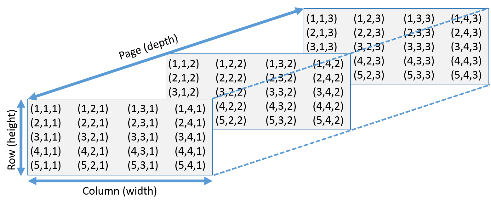![](http://www.socr.umich.edu/people/dinov/2017/Spring/DSPA_HS650/images/R_MatrixArrays_Diagram.png):	
#' 	
#' 	
ar<-array(1:24, dim=c(3, 4, 2))	
ar	
ar[2, 3, 1]	
ar[2, ,1]	
#' 	
#' 	
#' * In General, multi-dimensional arrays are called "tensors" (of order=number of dimensions).	
#' 	
#' Other useful functions are:	
#' 	
#' * `matrix(x, nrow=, ncol=)`: creates matrix elements of `nrow` rows and `ncol` columns.	
#' * `factor(x, levels=)`: encodes a vector `x` as a factor. 	
#' * `gl(n, k, length=n*k, labels=1:n)`: generate levels (factors) by specifying the pattern of their levels.	
#' *k* is the number of levels, and *n* is the number of replications.	
#' * `expand.grid()`: a data frame from all combinations of the supplied vectors or factors.	
#' * `rbind()` combine arguments by rows for matrices, data frames, and others	
#' * `cbind()` combine arguments by columns for matrices, data frames, and others	
#' 	
#' 	
#' ### Input/Output (I/O)	
#' 	
#' The first pair of functions we will talk about are `save()` and `load()`, which write and import objects between the current `R` environment RAM memory and long term storage, e.g., hard drive, Cloud storage, SSD, etc. The script below demonstrates the basic export and import operations with simple data. Note that we saved the data in `Rdata` (`Rda`) format.	
#' 	
#' 	
x <- seq(1, 10, by=0.5)	
y <- list(a = 1, b = TRUE, c = "oops")	
save(x, y, file="xy.RData")	
load("xy.RData")	
#' 	
#' 	
#' There are two basic functions `data(x)` and `library(x)` that load specified data sets and `R` packages, respectively. The `R` *base* library is always loaded by default. However, add-on libraries need to be *installed* first and then *imported* (loaded) in the working environment before functions and objects in these libraries are accessible.	
#' 	
#' 	
data("iris")	
summary(iris)	
	
library(base)	
#' 	
#' 	
#' **read.table(file)** reads a file in table format and creates a  data frame from it. The default separator `sep=""` is any whitespace. Use `header=TRUE` to read the first line as a header of column names. Use `as.is=TRUE` to prevent character vectors from being converted to factors. Use `comment.char=""` to prevent `"#"` from being interpreted as a comment. Use `skip=n` to skip `n` lines before reading data.  See the help for options on row naming, NA treatment, and others.	
#' 	
#' The example below uses `read.table()` to parse and load an ASCII text file containing a simple dataset, which is available on the [supporting canvas data archive](https://umich.instructure.com/courses/38100/files).	
#' 	
#' 	
data.txt<-read.table("https://umich.instructure.com/files/1628628/download?download_frd=1", header=T, as.is = T) # 01a_data.txt	
summary(data.txt)	
#' 	
#' 	
#' When using `R` to access (read/write) data on a Cloud web service, like [Instructure/Canvas](https://umich.instructure.com/courses/38100/files/folder/Case_Studies) or GoogleDrive/GDrive, mind that the direct URL reference to the raw file will be different from the URL of the pointer to the file that can be rendered in the browser window. For instance,	
#' 	
#'  - This [GDrive TXT file, *1Zpw3HSe-8HTDsOnR-n64KoMRWYpeBBek* (01a_data.txt)](https://drive.google.com/open?id=1Zpw3HSe-8HTDsOnR-n64KoMRWYpeBBek),	
#'  - [Can be downloaded and ingested in `R` via this separate URL](https://drive.google.com/uc?export=download&id=1Zpw3HSe-8HTDsOnR-n64KoMRWYpeBBek).	
#'  - While the file reference is unchanged (*1Zpw3HSe-8HTDsOnR-n64KoMRWYpeBBek*), note the change of syntax from viewing the file in the browser, **open?id=**, to auto-downloading the file for `R` processing, **uc?export=download&id=**.	
#' 	
#' 	
dataGDrive.txt<-read.table("https://drive.google.com/uc?export=download&id=1Zpw3HSe-8HTDsOnR-n64KoMRWYpeBBek", header=T, as.is = T) # 01a_data.txt	
summary(dataGDrive.txt)	
#' 	
#' 	
#' **read.csv("filename", header=TRUE)** is identical to `read.table()` but with defaults set for reading comma-delimited files.	
#' 	
#' 	
data.csv<-read.csv("https://umich.instructure.com/files/1628650/download?download_frd=1", header = T)  # 01_hdp.csv	
summary(data.csv)	
#' 	
#' 	
#' **read.delim("filename", header=TRUE)** is very similar to the first two. However, it has defaults set for reading tab-delimited files.	
#' 	
#' Also we have `read.fwf(file, widths, header=FALSE, sep="\t", as.is=FALSE)` to read a table of fixed width formatted data into a data frame.	
#' 	
#' **match(x, y)** returns a vector of the positions of (first) matches of its first argument in its second. For a specific element in `x` if no element matches it in `y`, then the output would be `NA`.	
#' 	
#' 	
match(c(1, 2, 4, 5), c(1, 4, 4, 5, 6, 7))	
#' 	
#' 	
#' **save.image(file)** saves all objects in the current workspace.	
#' 	
#' **write.table**(x, file="", row.names=TRUE, col.names=TRUE, sep="") prints x after converting to a data frame and stores it into a specified file. If `quote` is TRUE, character or factor columns are surrounded by quotes ("). `sep` is the field separator. `eol` is the end-of-line separator. `na` is the string for missing values. Use `col.names=NA` to add a blank column header to get the column headers aligned correctly for spreadsheet input.	
#' 	
#' Most of the I/O functions have a file argument. This can often be a character string naming a file or a connection. `file=""` means the standard input or output. Connections can include files, pipes, zipped files, and `R` variables.	
#' 	
#' On windows, the file connection can also be used with `description = "clipboard"`. To read a table copied from Excel, use `x <- read.delim("clipboard")`	
#' 	
#' To write a table to the clipboard for Excel, use `write.table(x, "clipboard", sep="\t", col.names=NA)`	
#' 	
#' For database interaction, see packages RODBC, DBI, RMySQL, RPgSQL, and ROracle, as well as packages XML, hdf5, netCDF for reading other file formats. We will talk about some of them in later chapters.	
#' 	
#' *Note*, an alternative library called `rio` handles import/export of multiple data types with simple syntax.	
#' 	
#' ### Slicing and extracting data		
#' 	
#' The following table summarizes the basic vector indexing operations.	
#' 	
#' Expression     |Explanation	
#' -------------- |-----------	
#' `x[n]`	       |nth element	
#' `x[-n]`	|all but the nth element	
#' `x[1:n]`|	first n elements	
#' `x[-(1:n)]`	|elements from n+1 to the end	
#' `x[c(1, 4, 2)]`|	specific elements	
#' `x["name"]`	 |element named "name"	
#' `x[x > 3]`	|all elements greater than 3	
#' `x[x > 3 & x < 5]`|	all elements between 3 and 5	
#' `x[x %in% c("a", "and", "the")]`| elements in the given set	
#' 	
#' Indexing lists are similar but not identical to indexing vectors.	
#' 	
#' Expression     |Explanation	
#' -------------- |-----------	
#' `x[n]`	|list with n elements 	
#' `x[[n]]`|	nth element of the list	
#' `x[["name"]]`| element of the list named "name" 		
#' 	
#' Indexing for *matrices* and higher dimensional *arrays* (*tensors*) derive from vector indexing.	
#' 	
#' Expression     |Explanation	
#' -------------- |-----------	
#' `x[i, j]`|	element at row i, column j 	
#' `x[i, ]` |	row i	
#' `x[, j]`	|column j 	
#' `x[, c(1, 3)]`| columns 1 and 3 	
#' `x["name", ]`| row named "name"	
#' 	
#' ### Variable conversion		
#' 	
#' The following functions represent simple examples of convert data types:	
#' 	
#' `as.array(x)`, `as.data.frame(x)`, `as.numeric(x)`, `as.logical(x)`, `as.complex(x)`, `as.character(x)`, ...	
#' 	
#' Typing `methods(as)` in the console will generate a complete list for variable conversion functions. 	
#' 	
#' ### Variable information		
#' 	
#' The following functions verify if the input is of a specific data type:	
#' 	
#' `is.na(x)`, `is.null(x)`, `is.array(x)`, `is.data.frame(x)`, `is.numeric(x)`, `is.complex(x)`, `is.character(x)`, ...	
#' 	
#' For a complete list, type `methods(is)` in the `R` console. The outputs for these functions are objects, either single values (`TRUE` or `FALSE`), or objects of the same dimensions as the inputs containing a Boolean `TRUE` or `FALSE` element for each entry in the dataset.	
#' 	
#' **length(x)** gives us the number of elements in `x`.	
#' 	
x<-c(1, 3, 10, 23, 1, 3)	
length(x)	
is.na(x)	
is.vector(x)	
#' 	
#' 	
#' **dim(x)** retrieves or sets the dimension of an array and **length(y)** reports the length of a list or a vector.	
#' 	
#' 	
x<-1:12	
length(x)	
dim(x)<-c(3, 4)	
x	
#' 	
#' 	
#' **dimnames(x)** retrieves or sets the dimension names of an object. For higher dimensional objects like matrices or arrays we can combine `dimnames()` with a list.	
#' 	
#' 	
dimnames(x)<-list(c("R1", "R2", "R3"), c("C1", "C2", "C3", "C4"))	
x	
#' 	
#' 	
#' **nrow(x)** and **ncol(x)** report the number of rows and number of columns or a matrix.	
#' 	
#' 	
nrow(x)	
ncol(x)	
#' 	
#' 	
#' **class(x)** gets or sets the class of $x$. Note that we can use `unclass(x)` to remove the class attribute of $x$. 	
#' 	
#' 	
class(x)	
class(x)<-"myclass"	
x<-unclass(x)	
x	
#' 	
#' 	
#' **attr(x, which)** gets or sets the attribute `which` of $x$.	
#' 	
#' 	
attr(x, "class")	
attr(x, "dim")<-c(2, 6)	
x	
#' 	
#' 	
#' The above script shows that applying `unclass` to $x$ sets its class to `NULL`.	
#' 	
#' **attributes(obj)** gets or sets the list of *attributes* of an object.	
#' 	
#' 	
attributes(x) <- list(mycomment = "really special", dim = 3:4, 	
   dimnames = list(LETTERS[1:3], letters[1:4]), names = paste(1:12))	
x	
#' 	
#' 	
#' ### Data selection and manipulation	
#' 	
#' In this section, we will introduce some data manipulation functions. In addition, tools from `dplyr` provide easy dataset manipulation routines.	
#' 	
#' **which.max(x)** returns the index of the greatest element (max) of $x$, **which.min(x)** returns the index of the smallest element (min) of $x$, and **rev(x)** reverses the elements of $x$.	
#' 	
#' 	
x<-c(1, 5, 2, 1, 10, 40, 3)	
which.max(x)	
which.min(x)	
rev(x)	
#' 	
#' 	
#' **sort(x)** sorts the elements of $x$ in increasing order. To sort in decreasing order we can use `rev(sort(x))`.	
#' 	
#' 	
sort(x)	
rev(sort(x))	
#' 	
#' 	
#' **cut(x, breaks)** divides $x$ into intervals with the same length (sometimes factors). The optional parameter `breaks` specifies the number of cut intervals or a vector of cut points. `cut` divides the range of $x$ into intervals coding the values in $x$ according to the intervals they fall into.	
#' 	
#' 	
x	
cut(x, 3)	
cut(x, c(0, 5, 20, 30))	
#' 	
#' 	
#' **which(x == a)** returns a vector of the indices of $x$ if the comparison operation is true. For example, it returns the value $i$, if $x[i]== a$ is TRUE. Thus, the argument of this function (like `x==a`) must be a Boolean variable.	
#' 	
#' 	
x	
which(x==2)	
#' 	
#' 	
#' **na.omit(x)** suppresses the observations with missing data (`NA`). It suppresses the corresponding line if $x$ is a matrix or a data frame. **na.fail(x)** returns an error message if $x$ contains at least one `NA`.	
#' 	
#' 	
df<-data.frame(a=1:5, b=c(1, 3, NA, 9, 8))	
df	
na.omit(df)	
#' 	
#' 	
#' **unique(x)** If $x$ is a vector or a data frame, it returns a similar object suppressing the duplicate elements.	
#' 	
#' 	
df1<-data.frame(a=c(1, 1, 7, 6, 8), b=c(1, 1, NA, 9, 8))	
df1	
unique(df1)	
#' 	
#'  	
#' **table(x)** returns a table with the different values of $x$ and their frequencies (typically used for integer or factor variables). The corresponding **prop.table()** function transforms these raw frequencies to relative frequencies (proportions, marginal mass).	
#' 	
#' 	
v<-c(1, 2, 4, 2, 2, 5, 6, 4, 7, 8, 8)	
table(v)	
prop.table(v)	
#' 	
#' 	
#' **subset(x, ...)** returns a selection of $x$ with respect to the specified criteria `...`. Typically `...` are comparisons like `x$V1 < 10`. If $x$ is a data frame, the option `select=` allows using a negative sign $-$ to indicate values to keep or drop from the object.	
#' 	
#' 	
sub <- subset(df1, df1$a>5)	
sub	
sub <- subset(df1, select=-a)	
sub	
	
## Subsampling	
x <- matrix(rnorm(100), ncol = 5)	
y <- c(1, seq(19))	
	
z <- cbind(x, y)	
	
z.df <- data.frame(z)	
z.df	
	
names(z.df)	
# subsetting rows	
z.sub <- subset(z.df, y > 2 & (y<10 | V1>0))	
z.sub	
	
z.sub1 <- z.df[z.df$y == 1, ]	
z.sub1	
z.sub2 <- z.df[z.df$y %in% c(1, 4), ]	
z.sub2	
	
# subsetting columns	
z.sub6 <- z.df[, 1:2]	
z.sub6	
#' 	
#' 	
#' **sample(x, size)** resamples randomly, without replacement, *size* elements in the vector $x$. The option `replace = TRUE` allows resampling with replacement.	
#' 	
#' 	
df1 <- data.frame(a=c(1, 1, 7, 6, 8), b=c(1, 1, NA, 9, 8))	
sample(df1$a, 20, replace = T)	
#' 	
#' 	
#' 	
#' ## Mathematics, Statistics, and Optimization	
#' 	
#' Many mathematical functions, statistical summaries, and function optimizers will be discussed throughout the book. Below are the very basic functions to keep in mind.	
#' 	
#' ### Math Functions		
#' 	
#' Basic math functions like `sin`, `cos`, `tan`, `asin`, `acos`, `atan`, `atan2`, `log`, `log10`, `exp` and "set" functions `union(x, y)`, `intersect(x, y)`, `setdiff(x, y)`, `setequal(x, y)`, `is.element(el, set)` are available in R.	
#' 	
#' `lsf.str("package:base")` displays all base functions built in a specific `R` package (like `base`).	
#' 	
#' This table summarizes the core functions for most basic `R` for calculations.	
#' 	
#' Expression           |Explanation	
#' ---------------------|-------------------------------------------------------------	
#' `choose(n, k)`| computes the combinations of k events among n repetitions. Mathematically it equals to  $\frac{n!}{[(n-k)!k!]}$	
#' `max(x)`| maximum of the elements of x	
#' `min(x)`| minimum of the elements of x 	
#' `range(x)`| minimum and maximum of the elements of x 	
#' `sum(x)`| sum of the elements of x	
#' `diff(x)`| lagged and iterated differences of vector x	
#' `prod(x)`| product of the elements of x 	
#' `mean(x)`| mean of the elements of x 	
#' `median(x)`| median of the elements of x	
#' `quantile(x, probs=)`| sample quantiles corresponding to the given probabilities (defaults to 0, .25, .5, .75, 1)	
#' `weighted.mean(x, w)`| mean of x with weights w	
#' `rank(x)`| ranks of the elements of x	
#' `var(x)` or `cov(x)`| variance of the elements of x (calculated on n>1). If x is a matrix or a data frame, the variance-covariance matrix is calculated	
#' `sd(x)`| standard deviation of x	
#' `cor(x)`| correlation matrix of x if it is a matrix or a data frame (1 if x is a vector)	
#' `var(x, y)` or `cov(x, y)`| covariance between x and y, or between the columns of x and those of y if they are matrices or data frames	
#' `cor(x, y)`| linear correlation between x and y, or correlation matrix if they are matrices or data frames	
#' `round(x, n)`| rounds the elements of x to n decimals	
#' `log(x, base)`| computes the logarithm of x with base base	
#' `scale(x)`| if x is a matrix, centers and reduces the data. Without centering use the option `center=FALSE`. Without scaling use `scale=FALSE` (by default center=TRUE, scale=TRUE)	
#' `pmin(x, y, ...)`| a vector whose i-th element is the minimum of x[i], y[i], . . .	
#' `pmax(x, y, ...)`| a vector whose i-th element is the maximum of x[i], y[i], . . .	
#' `cumsum(x)`| a vector which ith element is the sum from x[1] to x[i]	
#' `cumprod(x)`| id. for the product 	
#' `cummin(x)`| id. for the minimum 	
#' `cummax(x)`| id. for the maximum	
#' `Re(x)`|real part of a complex number	
#' `Im(x)`| imaginary part of a complex number	
#' `Mod(x)`| modulus. `abs(x)` is the same	
#' `Arg(x)`| angle in radians of the complex number	
#' `Conj(x)`| complex conjugate	
#' `convolve(x, y)`| compute several types of convolutions of two sequences	
#' `fft(x)`| Fast Fourier Transform of an array	
#' `mvfft(x)`| FFT of each column of a matrix	
#' `filter(x, filter)`| applies linear filtering to a univariate time series or to each series separately of a multivariate time series	
#' 	
#' Note: many math functions have a logical parameter `na.rm=TRUE` to specify missing data (`NA`) removal.	
#' 	
#' ### Matrix Operations		
#' 	
#' The following table summarizes basic operation functions. We will discuss this topic in detail in [Chapter 3 (Linear Algebra, Matrix Computing, and Regression Modeling)](https://socr.umich.edu/DSPA2/DSPA2_notes/03_LinearAlgebraMatrixComputingRegression.html).	
#' 	
#' Expression    |Explanation	
#' --------------|-------------------------------------------------------------------	
#' `t(x)`| transpose	
#' `diag(x)`| diagonal	
#' `%*%`| matrix multiplication	
#' `solve(a, b)`| solves `a %*% x = b` for x	
#' `solve(a)`| matrix inverse of a	
#' `rowsum(x)`| sum of rows for a matrix-like object. `rowSums(x)` is a faster version	
#' `colsum(x)`, `colSums(x)`| id. for columns 	
#' `rowMeans(x)`| fast version of row means 	
#' `colMeans(x)`| id. for columns	
#' 	
#' 	
mat1 <- cbind(c(1, -1/5), c(-1/3, 1))	
mat1.inv <- solve(mat1)	
	
mat1.identity <- mat1.inv %*% mat1	
mat1.identity	
b <- c(1, 2)	
x <- solve (mat1, b)	
x	
#' 	
#' 	
#' ### Optimization and model fitting		
#' 	
#'  - **optim(par, fn, method = c("Nelder-Mead", "BFGS", "CG", "L-BFGS-B", "SANN"))** general-purpose optimization; `par` is initial values, `fn` is a function to optimize (normally minimize).	
#'  - **nlm(f, p)** minimize function fusing a Newton-type algorithm with starting values p.	
#'  - **lm(formula)** fit linear models; `formula` is typically of the form `response ~ termA + termB + ...`; use `I(x*y) + I(x^2)` for terms made of nonlinear components.	
#'  - **glm(formula, family=)** fit generalized linear models, specified by giving a symbolic description of the linear predictor and a description of the error distribution; `family` is a description of the error distribution and link function to be used in the model; see `?family`.	
#'  - **nls(formula)** nonlinear least-squares estimates of the nonlinear model parameters.	
#'  - **approx(x, y=)** linearly interpolate given data points; $x$ can be an $xy$ plotting structure.	
#'  - **spline(x, y=)** cubic spline interpolation.	
#'  - **loess(formula)** (locally weighted scatterplot smoothing) fit a polynomial surface using local fitting.	
#' 	
#' Many of the formula-based modeling functions have several common arguments:	
#' 	
#' `data=` the data frame for the formula variables, `subset=` a subset of variables used in the fit, `na.action=` action for missing values: `"na.fail"`, `"na.omit"`, or a function. 	
#' 	
#' The following generics often apply to model fitting functions:	
#' 	
#'  - `predict(fit, ...)` predictions from fit based on input data.	
#'  - `df.residual(fit)` returns the number of residual degrees of freedom. 	
#'  - `coef(fit)` returns  the  estimated  coefficients  (sometimes  with  their standard-errors). 	
#'  - `residuals(fit)` returns the residuals.	
#'  - `deviance(fit)` returns the deviance.	
#'  - `fitted(fit)` returns the fitted values.	
#'  - `logLik(fit)` computes the logarithm of the likelihood and the number of parameters.	
#'  - `AIC(fit)` computes the Akaike information criterion (AIC).	
#' 	
#' ### Statistics		
#' 	
#'  - **aov(formula)** analysis of variance model.	
#'  - **anova(fit, ...)** analysis of variance (or deviance) tables for one or more fitted model objects.	
#'  - **density(x)** kernel density estimates of x.	
#' 	
#' Other functions include: `binom.test()`, 	`pairwise.t.test()`, 	`power.t.test()`, `prop.test()`, `t.test()`, ... use `help.search("test")` to see details.	
#' 	
#' ### Distributions	
#' 	
#' The [Probability Distributome Project](http://distributome.org) provides many details about univariate probability distributions. The [SOCR R Shiny Distribution Calculators](https://rcompute.nursing.umich.edu/DistributionCalculator/) and the [SOCR Bivariate and Trivariate Interactive Graphical Calculators](https://socr.umich.edu/HTML5/BivariateNormal/) provide additional demonstrations of multivariate probability distribution.	
#' 	
#' In `R`, there are four complementary functions supporting each probability distribution. For *Normal distribution*, these four functions are `dnorm()` - density, `pnorm()` - distribution function, `qnorm()` - quantile function, and `rnorm()` - random generating function. For *Poisson distribution*, the corresponding functions are `dpois()`, `ppois()`, `qpois()`, and `rpois()`.	
#' 	
#' The table below shows the invocation syntax for generating random samples from a number of different probability distributions.	
#' 	
#' Expression                       |Explanation	
#' ---------------------------------|-----------	
#' `rnorm(n, mean=0, sd=1)`| Gaussian (normal)	
#' `rexp(n, rate=1)`| exponential	
#' `rgamma(n, shape, scale=1)`| gamma	
#' `rpois(n, lambda)`| Poisson	
#' `rweibull(n, shape, scale=1)`| Weibull 	
#' `rcauchy(n, location=0, scale=1)`| Cauchy 	
#' `rbeta(n, shape1, shape2)`| beta	
#' `rt(n, df)`| Student's (t)	
#' `rf(n, df1, df2)`| Fisher's (F) (df1, df2)	
#' `rchisq(n, df)`| Pearson rbinom(n, size, prob) binomial 	
#' `rgeom(n, prob)`| geometric	
#' `rhyper(nn, m, n, k)`| hypergeometric 	
#' `rlogis(n, location=0, scale=1)`| logistic	
#' `rlnorm(n, meanlog=0, sdlog=1)`| lognormal 	
#' `rnbinom(n, size, prob)`| negative binomial 	
#' `runif(n, min=0, max=1)`| uniform	
#' `rwilcox(nn, m, n)`, `rsignrank(nn, n)`| Wilcoxon's statistics	
#' 	
#' Obviously, replacing the first letter `r` with `d`, `p` or `q` would reference the corresponding probability density (`dfunc(x, ...)`), the cumulative probability density (`pfunc(x, ...)`), and the value of quantile (`qfunc(p, ...)`, with $0 < p < 1$).	
#' 	
#' 	
#' ## Advanced Data Processing		
#' 	
#' In this section, we will introduce some useful functions that are useful in many data analytic protocols. The family of `*apply()` functions act on lists, arrays, vectors, data frames and other objects.	
#' 	
#' **apply(X, INDEX, FUN=)** returns a vector or array or list of values obtained by applying a function `FUN` to margins (`INDEX=1` means row, `INDEX=2` means column) of $X$. Additional options may be specified after the `FUN` argument.	
#' 	
#' 	
df1	
apply(df1, 2, mean, na.rm=T)	
#' 	
#' 	
#' **lapply(X, FUN)** applies `FUN` to each member of the list $X$. If $X$ is a data frame then it will apply the `FUN` to each column and return a list. 	
#' 	
#' 	
lapply(df1, mean, na.rm=T)	
lapply(list(a=c(1, 23, 5, 6, 1), b=c(9, 90, 999)), median)	
#' 	
#' 	
#' **tapply(X, INDEX, FUN=)** applies `FUN` to each cell of a ragged array given by $X$ with indexes equals to `INDEX`. Note that $X$ is an atomic object, typically a vector.	
#' 	
#' 	
# v<-c(1, 2, 4, 2, 2, 5, 6, 4, 7, 8, 8)	
v	
fac <- factor(rep(1:3, length = 11), levels = 1:3)	
table(fac)	
tapply(v, fac, sum)	
#' 	
#' 	
#' **by(data, INDEX, FUN)** applies  `FUN` to data frame data subsetted by INDEX. In this example, we apply the `sum` function using column 1 (`a`) as an index.	
#' 	
#' 	
by(df1, df1[, 1], sum)	
#' 	
#' 	
#' **merge(a, b)** merges two data frames by common columns or row names. We can use option `by=` to specify the index column.	
#' 	
#' 	
df2<-data.frame(a=c(1, 1, 7, 6, 8), c=1:5)	
df2	
df3<-merge(df1, df2, by="a")	
df3	
#' 	
#' 	
#' **xtabs(a ~ b, data=x)** reports specific factorized contingency tables. The example below uses the [1973 UC Berkeley admissions dataset](https://www.jstor.org/stable/1739581) to report gender-by-status breakdown.	
#' 	
#' 	
DF <- as.data.frame(UCBAdmissions)	
##  'DF' is a data frame with a grid of the factors and the counts	
## in variable 'Freq'.	
DF	
## Nice for taking margins ...	
xtabs(Freq ~ Gender + Admit, DF)	
## And for testing independence ...	
summary(xtabs(Freq ~ ., DF))	
#' 	
#' 	
#' **aggregate(x, by, FUN)** splits the data frame $x$ into subsets, computes summary statistics for each part, and reports the results. `by` is a list of grouping elements, each of which has the same length as the variables in $x$. For example, we can apply the function `sum` to the data frame `df3` subject to the index created by `list(rep(1:3, length=7))`.	
#' 	
#' 	
#' 	
list(rep(1:3, length=7))	
aggregate(df3, by=list(rep(1:3, length=7)), sum)	
#' 	
#' 	
#' **stack(x, ...)** transforms data stored as separate columns in a data frame, or list, into a single column vector; **unstack(x, ...)** is the inverse of `stack()`.	
#' 	
#' 	
stack(df3)	
unstack(stack(df3))	
#' 	
#' 	
#' **reshape(x, ...)** reshapes a data frame between *wide* format, with repeated measurements in separate columns of the same record, and *long* format, with the repeated measurements in separate records. We can specify the transformation direction, `direction="wide"` or `direction="long"`.	
#' 	
#' 	
df4 <- data.frame(school = rep(1:3, each = 4), class = rep(9:10, 6), 	
                  time = rep(c(1, 1, 2, 2), 3), score = rnorm(12))	
wide <- reshape(df4, idvar = c("school", "class"), direction = "wide")	
wide	
	
long <- reshape(wide, idvar = c("school", "class"), direction = "long")	
long	
#' 	
#' 	
#' <!---	
#' # See: http://stats.idre.ucla.edu/r/faq/how-can-i-reshape-my-data-in-r/	
#' 	
#' # wiki_url <- read_html("https://wiki.socr.umich.edu/index.php/SOCR_Data_PD_BiomedBigMetadata")	
#' #html_nodes(wiki_url, "#content")	
#' #pd_data <- html_table(html_nodes(wiki_url, "table")[[1]])	
#' #head(pd_data); summary(pd_data)	
#' long <- reshape(pd_data, 	
#'   varying = "Time", 	
#'   v.names = c("Time1", "Time2", "Time3", "Time4")  # colnames(pd_data)[-33],	
#'   times = "Time", 	
#'   direction = "long")	
#'   	
#' # arguments include 	
#' # (1) list of variable names that define the different times or metrics (varying), 	
#' # (2) the name we wish to give the variable containing these values in our long dataset (v.names), 	
#' # (3) the name we wish to give the variable describing the different times or metrics (timevar), 	
#' # (4) the values this variable will have (times), and 	
#' # (5) the end format for the data (direction)	
#' 	
#' wide <- reshape(pd_data, 	
#'   timevar = "Time",	
#'   idvar = colnames(pd_data)[-33],	
#'   direction = "wide")	
#'  	
#' # To reshape the PD dataset into a wide format, we will use the reshape function. The arguments we provide include 	
#' ### (1) *direction* = "wide" 	
#' ### (2) *timevar*, we indicate the variable that will define the multiple measurements per subject. 	
#' ### (3) *idvar* list the variables that should not vary within subject.	
#' --->	
#' 	
#' **Notes**	
#' 	
#'  - The $x$ in this function has to be longitudinal data.	
#'  - The call to `rnorm` used in reshape might generate different results for each call, unless `set.seed(1234)` is used to ensure reproducibility of random-number generation.	
#' 	
#' ### Strings		
#' 	
#' The following functions are useful for handling strings in `R`.	
#' 	
#' **paste(...)** and **paste0(...)**  concatenate vectors after converting the arguments to a vector of characters. There are several options, `sep=` to use a string to separate terms (a single space is the default), `collapse=` to separate "collapsed" results.	
#' 	
#' 	
a<-"today"	
b<-"is a good day"	
paste(a, b)	
paste(a, b, sep=", ")	
#' 	
#' 	
#' **substr(x, start, stop)** substrings in a character vector. Using `substr(x, start, stop) <- value`, it can also assign values (with the same length) to part of a string.	
#' 	
#' 	
a<-"When the going gets tough, the tough get going!"	
substr(a, 10, 40)	
## [1] "going gets tough, the tough get"	
substr(a, 1, 9)<-"........."	
a	
#' 	
#' 	
#' Note that characters at `start` and `stop` indexes are inclusive in the output.	
#' 	
#' **strsplit(x, split)** splits $x$ according to the substring split. Use `fixed=TRUE` for non-regular expressions.	
#' 	
#' 	
strsplit("a.b.c", ".", fixed = TRUE)	
#' 	
#' 	
#' **grep(pattern, x)** searches for pattern matches within $x$ and returns a vector of the indices of the elements of $x$ that had a match. Use regular expressions for `pattern`(unless `fixed=TRUE`), see `?regex` for details.	
#' 	
#' 	
letters	
grep("[a-z]", letters)	
#' 	
#' 	
#' **gsub(pattern, replacement, x)** replaces matching patterns in $x$, allowing for use of regular expression matching; **sub()** is the same but it only replaces the first occurrence of the matched pattern.	
#' 	
#' 	
a<-c("e", 0, "kj", 10, ";")	
gsub("[a-z]", "letters", a)	
sub("[a-z]", "letters", a)	
#' 	
#' 	
#' **tolower(x)** converts strings to lowercase and **toupper(x)** converts to uppercase.	
#' 	
#' **match(x, table)** yields a vector of the positions of first matches for the elements of $x$ among `table`, `x %in% table` returns a logical vector.	
#' 	
#' 	
x<-c(1, 2, 10, 19, 29)	
match(x, c(1, 10))	
x %in% c(1, 10)	
#' 	
#' 	
#' **pmatch(x, table)** reports partial matches for the elements of $x$. 	
#' 	
#' **Dates and Times**	
#' 	
#' The class `Date` stores calendar dates, without times. `POSIXct()` has dates and times, including time zones. Comparisons (e.g. $>$), `seq()`, and `difftime()` are useful to compare dates. `?DateTimeClasses` gives more information, see also package `chron`.	
#' 	
#' The functions `as.Date(s)` and `as.POSIXct(s)` convert to the respective class; `format(dt)` converts to a string representation. The default string format is `2001-02-21`. These accept a second argument to specify a format for conversion. Some common formats are:	
#' 	
#' Formats           | Explanations	
#' ------------------|---------------------------------------------------------------	
#' `%a, %A`| Abbreviated and full weekday name.	
#' `%b, %B`| Abbreviated and full month name.	
#' `%d` |Day of the month (01 ... 31).	
#' `%H`| Hours (00 ... 23).	
#' `%I`| Hours (01 ... 12).	
#' `%j`| Day of year (001 ... 366).	
#' `%m`| Month (01 ... 12).	
#' `%M`| Minute (00 ... 59).	
#' `%p`| AM/PM indicator.	
#' `%S`| Second as a decimal number (00 ... 61).	
#' `%U`| Week (00 ... 53); the first Sunday as day 1 of week 1.	
#' `%w`| Weekday (0 ... 6, Sunday is 0).	
#' `%W`| Week (00 ... 53); the first Monday as day 1 of week 1.	
#' `%y`| Year without century (00 ... 99). Don't use it.	
#' `%Y`| Year with century.	
#' `%z` (output only.)| Offset from Greenwich; -0800 is 8 hours west of.	
#' `%Z` (output only.)| Time zone as a character string (empty if not available).	
#' 	
#' Where leading zeros are shown they will be used on output but are optional on input. See `?strftime` for details.	
#' 	
#' ## Basic Plotting		
#' 	
#' The following functions represent the basic plotting functions in `R`. Later, in [Chapter 2 (Visualization & EDA)](https://socr.umich.edu/DSPA2/DSPA2_notes/02_Vizualization_EDA.html), we will discuss more elaborate visualization in and exploratory data analytic strategies.	
#' 	
#'  - **plot(x)** plot of the values of x (on the y-axis) ordered on the x-axis.	
#'  - **plot(x, y)** bivariate plot of x (on the x-axis) and y (on the y-axis).	
#'  - **hist(x)** histogram of the frequencies of x.	
#'  - **barplot(x)** histogram of the values of x. Use `horiz=FALSE` for horizontal bars.	
#'  - **dotchart(x)** if x is a data frame, plots a Cleveland dot plot (stacked plots line-by-line and column-by-column).	
#'  - **pie(x)** circular pie-chart.	
#'  - **boxplot(x)** 'box-and-whiskers' plot.	
#'  - **sunflowerplot(x, y)** sunflowers plot with multiple leaves (‘petals’) such that overplotting is visualized instead of accidental and invisible.	
#'  - **stripplot(x)** plot  of  the  values  of  x on  a  line  (an  alternative  to `boxplot()` for small sample sizes).	
#'  - **coplot(x~y |  z)** bivariate plot of x and y for each value or interval of values of z.	
#'  - **interaction.plot (f1, f2, y)** if f1 and f2 are factors, plots the means of y (on the y-axis) with respect to the values of f1 (on the x-axis) and of f2 (different curves). The option `fun` allows you to choose the summary statistic of y (by default `fun=mean`).	
#'  - **matplot(x, y)** bivariate plot of the first column of x vs. the first one of y, the second one of x vs. the second one of y, etc.	
#'  - **fourfoldplot(x)** visualizes, with quarters of circles, the association between two dichotomous variables for different populations (x must be an array with dim=c(2, 2, k), or a matrix with dim=c(2, 2) if k = 1)	
#'  - **assocplot(x)** Cohen's Friendly graph shows the deviations from independence of rows and columns in a two dimensional contingency table.	
#'  - **mosaicplot(x)** "mosaic"" graph of the residuals from a log-linear regression of a contingency table.	
#'  - **pairs(x)** if x is a matrix or a data frame, draws all possible bivariate plots between the columns of x.	
#'  - **plot.ts(x)** if x is an object of class "ts", plot of x with respect to time, x may be multivariate but the series must have the same frequency and dates. Detailed examples are in **Chapter 17: Big Longitudinal Data Analysis**.	
#'  - **ts.plot(x)** id. but if x is multivariate the series may have different dates and must have the same frequency.	
#'  - **qqnorm(x)** quantiles of x with respect to the values expected under a normal law.	
#'  - **qqplot(x, y)** quantiles of y with respect to the quantiles of x.	
#'  - **contour(x, y, z)** contour plot (data are interpolated to draw the curves), x and y must be vectors and z must be a matrix so that `dim(z)=c(length(x), length(y))` (x and y may be omitted).	
#'  - **filled.contour(x, y, z)** areas between the contours are colored, and a legend of the colors is drawn as well.	
#'  - **image(x, y, z)** plotting actual data with colors.	
#'  - **persp(x, y, z)** plotting actual data in perspective view.	
#'  - **stars(x)** if x is a matrix or a data frame, it draws a graph with segments or a star where each row of x is represented by a star and the columns are the lengths of the segments.	
#'  - **symbols(x, y, ...)** draws, at the coordinates given by x and y, symbols (circles, squares, rectangles, stars, thermometers or "boxplots"") whose sizes, colors... are specified by supplementary arguments.	
#'  - **termplot(mod.obj)** plot of the (partial) effects of a regression model (`mod.obj`).	
#' 	
#' The following parameters are common to many plotting functions: 	
#' 	
#' Parameters  | Explanations	
#' ------------|--------------------------------------------------------------	
#' `add=FALSE`| if TRUE superposes the plot on the previous one (if it exists) 	
#' `axes=TRUE`| if FALSE does not draw the axes and the box	
#' `type="p"`| specifies the type of plot, "p": points, "l": lines, "b": points connected by lines, "o": id. But the lines are over the points, "h": vertical lines, "s": steps, the data are represented by the top of the vertical lines, "S": id. However, the data are represented at the bottom of the vertical lines	
#' `xlim=, ylim=`| specifies the lower and upper limits of the axes, for example with `xlim=c(1, 10)` or `xlim=range(x)`	
#' `xlab=, ylab=`| annotates the axes, must be variables of mode character 	
#' `main=`| main title, must be a variable of mode character	
#' `sub=`| subtitle (written in a smaller font)	
#' 	
#' ### QQ Normal probability plot 	
#' 	
#' Let's look at one simple example - quantile-quantile probability plot. Suppose $X\sim N(0,1)$ and $Y\sim Cauchy$ represent the observed/raw and simulated/generated data for one feature (variable) in the data.	
#' 	
#' 	
# This commended example illustrates a linear model based approach (below is a more direct QQ-plot demonstration)	
# X_norm1 <- rnorm(1000)	
# X_norm2 <- rnorm(1000, m=-75, sd=3.7)	
# X_Cauchy <- rcauchy(1000)	
# 	
# # compare X to StdNormal distribution	
# # 	qqnorm(X, 	
# #          		main="Normal Q-Q Plot of the data", 	
# #          		xlab="Theoretical Quantiles of the Normal", 	
# #          		ylab="Sample Quantiles of the X (Normal) Data")	
# # 	qqline(X)	
# # 	qqplot(X, Y)	
# fit_norm_norm = lm(X_norm2 ~ X_norm1)	
# fit_norm_cauchy = lm(X_Cauchy ~ X_norm1)	
# 	
# # Get model fitted values	
# Fitted.Values.norm_norm <-  fitted(fit_norm_norm)	
# Fitted.Values.norm_cauchy <-  fitted(fit_norm_cauchy)	
#   	
# # Extract model residuals	
# Residuals.norm_norm <-  resid(fit_norm_norm)	
# Residuals.norm_cauchy <-  resid(fit_norm_cauchy)	
# 	
# # Compute the model standardized residuals from lm() object	
# Std.Res.norm_norm <- MASS::stdres(fit_norm_norm)  	
# Std.Res.norm_cauchy <- MASS::stdres(fit_norm_cauchy)  	
#   	
# # Extract the theoretical (Normal) quantiles	
# Theoretical.Quantiles.norm_norm <- qqnorm(Residuals.norm_norm, plot.it = F)$x	
# Theoretical.Quantiles.norm_cauchy <- qqnorm(Residuals.norm_cauchy, plot.it = F)$x	
#   	
# qq.df.norm_norm <- data.frame(Std.Res.norm_norm, Theoretical.Quantiles.norm_norm)	
# qq.df.norm_cauchy <- data.frame(Std.Res.norm_cauchy, Theoretical.Quantiles.norm_cauchy)	
# 	
# qq.df.norm_norm %>% 	
#   plot_ly(x = ~Theoretical.Quantiles.norm_norm) %>% 	
#     add_markers(y = ~Std.Res.norm_norm, name="Normal(0,1) vs. Normal(-75, 3.7) Data") %>%	
#     add_lines(x = ~Theoretical.Quantiles.norm_norm, y = ~Theoretical.Quantiles.norm_norm, 	
#               mode = "line", name = "Theoretical Normal", line = list(width = 2)) %>% 	
#     layout(title = "Q-Q Normal Plot", legend = list(orientation = 'h'))	
# 	
# # Normal vs. Cauchy	
# qq.df.norm_cauchy %>% 	
#   plot_ly(x = ~Theoretical.Quantiles.norm_cauchy) %>% 	
#     add_markers(y = ~Std.Res.norm_cauchy, name="Normal(0,1) vs. Cauchy Data") %>%	
#     add_lines(x = ~Theoretical.Quantiles.norm_norm, y = ~Theoretical.Quantiles.norm_norm, 	
#               mode = "line", name = "Theoretical Normal", line = list(width = 2)) %>% 	
#     layout(title = "Normal vs. Cauchy Q-Q Plot", legend = list(orientation = 'h'))	
	
# Q-Q plot data (X) vs. simulation(Y)	
# 	
# myQQ <- function(x, y, ...) {	
#   #rang <- range(x, y, na.rm=T)	
#   rang <- range(-4, 4, na.rm=T)	
#   qqplot(x, y, xlim=rang, ylim=rang)	
# }	
# 	
# myQQ(X, Y) # where the Y is the newly simulated data for X	
# qqline(X)	
	
# Sample different number of observations from all the 3 processes	
X_norm1 <- rnorm(500)	
X_norm2 <- rnorm(1000, m=-75, sd=3.7)	
X_Cauchy <- rcauchy(1500)	
	
# estimate the quantiles (scale the values to ensure measuring-unit invariance of both processes)	
qX_norm1 <- quantile(scale(X_norm1), probs = seq(from=0.01, to=0.99, by=0.01))	
qX_norm2 <- quantile(scale(X_norm2), probs = seq(from=0.01, to=0.99, by=0.01))	
qq.df.norm_norm <- data.frame(qX_norm1, qX_norm2)	
	
# Normal(0,1) vs. Normal(-75, 3.7)	
qq.df.norm_norm %>% 	
  plot_ly(x = ~qX_norm1) %>% 	
    add_markers(y = ~qX_norm2, name="Normal(0,1) vs. Normal(-75, 3.7) Data") %>%	
    add_lines(x = ~qX_norm1, y = ~qX_norm1, 	
              mode = "line", name = "Theoretical Normal", line = list(width = 2)) %>% 	
    layout(title = "Q-Q Normal Plot", legend = list(orientation = 'h'))	
	
# Normal(0,1) vs. Cauchy	
qX_norm1 <- quantile(X_norm1, probs = seq(from=0.01, to=0.99, by=0.01))	
qX_Cauchy <- quantile(X_Cauchy, probs = seq(from=0.01, to=0.99, by=0.01))	
qq.df.norm_cauchy <- data.frame(qX_norm1, qX_Cauchy)	
	
qq.df.norm_cauchy %>% 	
  plot_ly(x = ~qX_norm1) %>% 	
    add_markers(y = ~qX_Cauchy, name="Normal(0,1) vs. Cauchy Data") %>%	
    add_lines(x = ~qX_norm1, y = ~qX_norm1, 	
              mode = "line", name = "Theoretical Normal", line = list(width = 2)) %>% 	
    layout(title = "Normal vs. Cauchy Q-Q Plot", legend = list(orientation = 'h'))	
#' 	
#' 	
#' ### Low-level plotting commands	
#' 	
#'  - **points(x, y)** adds points (the option `type=` can be used)	
#'  - **lines(x, y)** id. but with lines	
#'  - **text(x, y, labels, ...)** adds text given by labels at coordinates (x, y). Typical use: `plot(x, y, type="n"); text(x, y, names)`	
#'  - **mtext(text, side=3, line=0, ...)** adds text given by text in the margin specified by side (see `axis()` below); line specifies the line from the plotting area.	
#'  - **segments(x0, y0, x1, y1)** draws lines from points `(x0, y0)` to points `(x1, y1)`	
#'  - **arrows(x0, y0, x1, y1, angle= 30, code=2)** id. With arrows at points `(x0, y0)`, if `code=2`. The arrow is at point `(x1, y1)`, if `code=1`. Arrows are at both if `code=3`. Angle controls the angle from the shaft of the arrow to the edge of the arrow head.	
#'  - **abline(a, b)** draws a line of slope `b` and intercept `a`.	
#'  - **abline(h=y)** draws a horizontal line at ordinate y.	
#'  - **abline(v=x)** draws a vertical line at abscissa x. 	
#'  - **abline(lm.obj)** draws the regression line given by `lm.obj`.  abline(h=0, col=2) #color (col) is often used	
#'  - **rect(x1, y1, x2, y2)** draws a rectangle whose left, right, bottom, and top limits are x1, x2, y1, and y2, respectively.	
#'  - **polygon(x, y)** draws a polygon linking the points with coordinates given by x and y.	
#'  - **legend(x, y, legend)** adds the legend at the point `(x, y)` with the symbols given by `legend`.	
#'  - **title()** adds a title and optionally a subtitle.	
#'  - **axis(side, vect)** adds an axis at the bottom (`side=1`), on the left (`side=2`), at the top (`side=3`), or on the right (`side=4`); `vect` (optional) gives the abscissa (or ordinates) where tick-marks are drawn.	
#'  - **rug(x)** draws the data x on the x-axis as small vertical lines.	
#'  - **locator(n, type="n", ...)** returns the coordinates `(x, y)` after the user has clicked n times on the plot with the mouse; also draws symbols (`type="p"`) or lines (`type="l"`) with respect to optional graphic parameters (...); by default nothing is drawn (`type="n"`).	
#' 	
#' ### General graphics parameters	
#' 	
#' These can be set globally with **par(...)**. Many can be passed as parameters to plotting commands.	
#' 	
#'  - **adj** controls text justification (`adj=0` left-justified, `adj=0.5` centered, `adj=1` right-justified).	
#'  - **bg** specifies the color of the background (ex. : `bg="red"`, `bg="blue"`, ...the list of the 657 available colors is displayed with `colors()`).	
#'  - **bty** controls the type of box drawn around the plot. Allowed values are: "o", "l", "7", "c", "u" ou "]" (the box looks like the corresponding character). If `bty="n"` the box is not drawn.	
#'  - **cex** a value controlling the size of texts and symbols with respect to the default. The following parameters have the same control for numbers on the axes-`cex.axis`, the axis labels-`cex.lab`, the title-`cex.main`, and the subtitle-`cex.sub`.	
#'  - **col** controls the color of symbols and lines. Use color names: "red", "blue" see `colors()` or as "#RRGGBB"; see `rgb()`, `hsv()`, `gray()`, and `rainbow()`; as for cex there are: `col.axis`, `col.lab`, `col.main`, `col.sub`.	
#'  - **font** an integer which controls the style of text (1: normal, 2: italics, 3: bold, 4: bold italics); as for cex there are: `font.axis`, `font.lab`, `font.main`, `font.sub`.	
#'  - **las** an integer which controls the orientation of the axis labels (0: parallel to the axes, 1: horizontal, 2: perpendicular to the axes, 3: vertical).	
#'  - **lty** controls the type of lines, can be an integer or string (1: "solid", 2: "dashed",  3: "dotted",  4: "dotdash",  5: "longdash",  6: "twodash", or a string of up to eight characters (between "0" and "9") which specifies alternatively the length, in points or pixels, of the drawn elements and the blanks, for example `lty="44"` will have the same effect than `lty=2`.	
#'  - **lwd** a numeric which controls the width of lines, default=1.	
#'  - **mar** a vector of 4 numeric values which control the space between the axes and the border of the graph of the form `c(bottom, left, top, right)`, the default values are `c(5.1, 4.1, 4.1, 2.1)`.	
#'  - **mfcol** a vector of the form `c(nr, nc)` which partitions the graphic window as a matrix of nr lines and nc columns, the plots are then drawn in columns.	
#'  - **mfrow** plots are drawn by row-by-row.	
#'  - **pch** controls the type of symbol, either an integer between 1 and 25, or any single character within "".	
#'  - **ts.plot(x)** id. but if x is multivariate the series may have different dates by x and y.	
#'  - **ps** an integer which controls the size in points of texts and symbols.	
#'  - **pty** a character, which specifies the type of the plotting region, "s": square, "m": maximal.	
#'  - **tck** a value which specifies the length of tick-marks on the axes as a fraction of the smallest of the width or height of the plot; if `tck=1` a grid is drawn.	
#'  - **tcl** a value which specifies the length of tick-marks on the axes as a fraction of the height of a line of text (by default `tcl=-0.5`).	
#'  - **xaxt** if `xaxt="n"` the x-axis is set but not drawn (useful in conjunction with `axis(side=1, ...)`).	
#'  - **yaxt** if `yaxt="n"` the y-axis is set but not drawn (useful in conjunction with `axis(side=2, ...)`).	
#' 	
#' Expression         | Explanation	
#' -------------------|--------------------------------	
#' **xyplot(y~x)**    | bivariate plots (with many functionalities). 	
#' **barchart(y~x)**  | histogram of the values of y with respect to those of x.	
#' **dotplot(y~x)**   | Cleveland dot plot (stacked plots line-by-line and column-by-column)	
#' **densityplot(~x)** |  density functions plot 	
#' **histogram(~x)** | histogram of the frequencies of x 	
#' **bwplot(y~x)**   | "box-and-whiskers" plot	
#' **qqmath(~x)**    | quantiles of x with respect to the values expected under a theoretical distribution	
#' **stripplot(y~x)**  | single dimension plot, x must be numeric, y may be a factor	
#' **qq(y~x)**         | quantiles to compare two distributions, x must be numeric, y may be numeric, character, or factor but must have two "levels"	
#' **splom(~x)**      | matrix of bivariate plots	
#' **parallel(~x)**   | parallel coordinates plot	
#' levelplot($z\sim x*y\|g1*g2$)   | colored plot of the values of z at the coordinates given by x and y (x, y and z are all of the same length)	
#' wireframe($z\sim x*y\|g1*g2$)   | 3d surface plot	
#' cloud($z\sim x*y\|g1*g2$)   | 3d scatter plot	
#' 	
#' In the normal Lattice formula, `y~x|g1*g2`, combinations of optional conditioning variables `g1` and `g2` plotted on separate panels. Lattice functions take many of the same arguments as base graphics plus also `data=` the data frame for the formula variables and `subset=` for subsetting. Use `panel=` to define a custom panel function (see `apropos("panel")` and `?lines`). Lattice functions return an object of class trellis and have to be printed to produce the graph. Use `print(xyplot(...))` inside functions where automatic printing doesn't work. Use `lattice.theme` and `lset` to change Lattice defaults.	
#' 	
#' 	
#' ## Basic `R` Programming	
#' 	
#' The standard setting for our **own function** is:	
#' 	
#' `function.name<-function(x) {`	
#' `       expr(an expression)`	
#' `       return(value)`	
#' `}` 	
#' 	
#' Where $x$ is the parameter in the expression. A simple example of this is:	
#' 	
#' 	
adding <- function(x=0, y=0) {	
  z<-x+y	
  return(z)	
}	
adding(x=5, y=10)	
#' 	
#' 	
#' **Conditions setting**: `if(cond) {expr}` or `if(cond) cons.expr else alt.expr`.	
#' 	
#' 	
x<-10	
if(x>10) z="T" else z="F"	
z	
#' 	
#' 	
#' Alternatively, `ifelse` represents a vectorized and extremely efficient conditional mechanism that provides one of the main advantages of `R`.	
#' 	
#' **For loop**: `for(var in seq) expr`.	
#' 	
#' 	
x<-c()	
for(i in 1:10) x[i]=i	
x	
#' 	
#' 	
#' **Other loops**: While loop: `while(cond) expr`, repeat: `repeat expr`. Applied to the innermost of nested loops: `break`, `next`. Use braces `{}` around statements.	
#' 	
#' **ifelse(test, yes, no)** returns a value with the same shape as test, filled with yes or no Boolean values.	
#' 	
#' **do.call(funname, args)** executes a function call from the name of the function and a list of arguments to be passed to it.	
#' 	
#' ## Data Simulation Primer	
#' 	
#' Before we demonstrate how to synthetically simulate data that resembles closely the characteristics of real observations from the same process, let's import some observed data for initial exploratory analytics.	
#' 	
#' Using the [SOCR Parkinson's Disease Case-study](https://wiki.socr.umich.edu/index.php/SOCR_Simulated_HELP_Data) available in the [Canvas Data Archive](https://umich.instructure.com/files/330397/download?download_frd=1), we can import some data and extract some descriptions of the [sample data (05_PPMI_top_UPDRS_Integrated_LongFormat1.csv)](https://umich.instructure.com/files/330397/download?download_frd=1). 	
#' 	
#' 	
PPMI <- read.csv("https://umich.instructure.com/files/330397/download?download_frd=1")	
# summary(PPMI)	
Hmisc::describe(PPMI)	
#' 	
#' 	
#' 	
#' 	
# data driven age estimates	
m  = round (mean(PPMI$Age), 2)	
sd = round(sd(PPMI$Age), 2)	
	
x.norm <- rnorm(n=200, m=m, sd=sd)	
# hist(x.norm, main='N(10, 20) Histogram')	
plot_ly(x = ~x.norm, type = "histogram") %>% 	
  layout(bargap=0.1, title=paste0('N(', m, ', ', sd, ') Histogram'))	
	
mean(PPMI$Age)	
sd(PPMI$Age)	
#' 	
#' 	
#' Next, we will simulate new synthetic data to match the properties/characteristics of the observed PPMI data (using `Uniform`, `Normal`, and `Poisson` distributions).	
#' 	
#' 	
# age m=62, sd=10	
	
# Demographics variables	
# Define number of subjects	
NumSubj <- 282	
NumTime <- 4	
	
# Define data elements	
# Cases	
Cases <- c(2, 3, 6, 7, 8, 10, 11, 12, 13, 14, 17, 18, 20, 21, 22, 23, 24, 25, 26, 28, 29, 30, 31, 32, 33, 34, 35, 37, 41, 42, 43, 44, 45, 53, 55, 58, 60, 62, 67, 69, 71, 72, 74, 79, 80, 85, 87, 90, 95, 97, 99, 100, 101, 106, 107, 109, 112, 120, 123, 125, 128, 129, 132, 134, 136, 139, 142, 147, 149, 153, 158, 160, 162, 163, 167, 172, 174, 178, 179, 180, 182, 192, 195, 201, 208, 211, 215, 217, 223, 227, 228, 233, 235, 236, 240, 245, 248, 250, 251, 254, 257, 259, 261, 264, 268, 269, 272, 273, 275, 279, 288, 289, 291, 296, 298, 303, 305, 309, 314, 318, 324, 325, 326, 328, 331, 332, 333, 334, 336, 338, 339, 341, 344, 346, 347, 350, 353, 354, 359, 361, 363, 364, 366, 367, 368, 369, 370, 371, 372, 374, 375, 376, 377, 378, 381, 382, 384, 385, 386, 387, 389, 390, 393, 395, 398, 400, 410, 421, 423, 428, 433, 435, 443, 447, 449, 450, 451, 453, 454, 455, 456, 457, 458, 459, 460, 461, 465, 466, 467, 470, 471, 472, 476, 477, 478, 479, 480, 481, 483, 484, 485, 486, 487, 488, 489, 492, 493, 494, 496, 498, 501, 504, 507, 510, 513, 515, 528, 530, 533, 537, 538, 542, 545, 546, 549, 555, 557, 559, 560, 566, 572, 573, 576, 582, 586, 590, 592, 597, 603, 604, 611, 619, 621, 623, 624, 625, 631, 633, 634, 635, 637, 640, 641, 643, 644, 645, 646, 647, 648, 649, 650, 652, 654, 656, 658, 660, 664, 665, 670, 673, 677, 678, 679, 680, 682, 683, 686, 687, 688, 689, 690, 692)	
	
# Imaging Biomarkers	
L_caudate_ComputeArea <- rpois(NumSubj, 600)	
L_caudate_Volume <- rpois(NumSubj, 800)	
R_caudate_ComputeArea <- rpois(NumSubj, 893)	
R_caudate_Volume <- rpois(NumSubj, 1000)	
L_putamen_ComputeArea <- rpois(NumSubj, 900)	
L_putamen_Volume <- rpois(NumSubj, 1400)	
R_putamen_ComputeArea <- rpois(NumSubj, 1300)	
R_putamen_Volume <- rpois(NumSubj, 3000)	
L_hippocampus_ComputeArea <- rpois(NumSubj, 1300)	
L_hippocampus_Volume <- rpois(NumSubj, 3200)	
R_hippocampus_ComputeArea <- rpois(NumSubj, 1500)	
R_hippocampus_Volume <- rpois(NumSubj, 3800)	
cerebellum_ComputeArea <- rpois(NumSubj, 16700)	
cerebellum_Volume <- rpois(NumSubj, 14000)	
L_lingual_gyrus_ComputeArea <- rpois(NumSubj, 3300)	
L_lingual_gyrus_Volume <- rpois(NumSubj, 11000)	
R_lingual_gyrus_ComputeArea <- rpois(NumSubj, 3300)	
R_lingual_gyrus_Volume <- rpois(NumSubj, 12000)	
L_fusiform_gyrus_ComputeArea <- rpois(NumSubj, 3600)	
L_fusiform_gyrus_Volume <- rpois(NumSubj, 11000)	
R_fusiform_gyrus_ComputeArea <- rpois(NumSubj, 3300)	
R_fusiform_gyrus_Volume <- rpois(NumSubj, 10000)	
	
Sex <- ifelse(runif(NumSubj)<.5, 0, 1)	
	
Weight <- as.integer(rnorm(NumSubj, 80, 10))	
	
Age <- as.integer(rnorm(NumSubj, 62, 10))	
	
# Diagnosis	
Dx <- c(rep("PD", 100), rep("HC", 100), rep("SWEDD", 82))	
	
# Genetics	
chr12_rs34637584_GT <- c(ifelse(runif(100)<.3, 0, 1), ifelse(runif(100)<.6, 0, 1), ifelse(runif(82)<.4, 0, 1))                              # NumSubj Bernoulli trials	
	
chr17_rs11868035_GT <- c(ifelse(runif(100)<.7, 0, 1), ifelse(runif(100)<.4, 0, 1), ifelse(runif(82)<.5, 0, 1))                              # NumSubj Bernoulli trials	
	
# Clinical          # rpois(NumSubj, 15) + rpois(NumSubj, 6)	
UPDRS_part_I <- c( ifelse(runif(100)<.7, 0, 1) + ifelse(runif(100) < .7, 0, 1), 	
	
ifelse(runif(100)<.6, 0, 1)+ ifelse(runif(100)<.6, 0, 1), 	
	
ifelse(runif(82)<.4, 0, 1)+ ifelse(runif(82)<.4, 0, 1) )	
	
UPDRS_part_II <- c(sample.int(20, 100, replace=T), sample.int(14, 100, replace=T), 	
	
sample.int(18, 82, replace=T) )	
	
UPDRS_part_III <- c(sample.int(30, 100, replace=T), sample.int(20, 100, replace=T), 	
	
           sample.int(25, 82, replace=T) )	
	
# Time: VisitTime - done automatically below in aggregator	
	
# Data (putting all components together)	
sim_PD_Data <- cbind(	
        rep(Cases, each= NumTime),                 # Cases	
        rep(L_caudate_ComputeArea, each= NumTime), # Imaging	
        rep(Sex, each= NumTime),                   # Demographics	
        rep(Weight, each= NumTime), 	
        rep(Age, each= NumTime), 	
        rep(Dx, each= NumTime),                    # Dx	
        rep(chr12_rs34637584_GT, each= NumTime),   # Genetics	
        rep(chr17_rs11868035_GT, each= NumTime), 	
        rep(UPDRS_part_I, each= NumTime),          # Clinical	
        rep(UPDRS_part_II, each= NumTime), 	
        rep(UPDRS_part_III, each= NumTime), 	
        rep(c(0, 6, 12, 18), NumSubj)                # Time	
)	
	
	
# Assign the column names	
	
colnames(sim_PD_Data) <- c(	
"Cases", 	
"L_caudate_ComputeArea", 	
"Sex", "Weight", "Age", 	
"Dx", "chr12_rs34637584_GT", "chr17_rs11868035_GT", 	
"UPDRS_part_I", "UPDRS_part_II", "UPDRS_part_III", 	
"Time"	
)	
	
# some QC	
summary(sim_PD_Data)	
dim(sim_PD_Data)	
head(sim_PD_Data)	
	
# hist(PPMI$Age, freq=FALSE, right=FALSE, ylim = c(0,0.05))	
# lines(density(as.numeric(as.data.frame(sim_PD_Data)$Age)), lwd=2, col="blue")	
# legend("topright", c("Raw Data", "Simulated Data"), fill=c("black", "blue"))	
	
x <- PPMI$Age	
fit <- density(as.numeric(as.data.frame(sim_PD_Data)$Age))	
	
plot_ly(x = x, type = "histogram", name = "Histogram (Raw Age)") %>% 	
    add_trace(x = fit$x, y = fit$y, type = "scatter", mode = "lines", 	
              fill = "tozeroy", yaxis = "y2", name = "Density (Simulated Age)") %>% 	
    layout(title='Observed and Simulated Ages', yaxis2 = list(overlaying = "y", side = "right"))	
	
	
# Save Results	
# Write out (save) the result to a file that can be shared	
write.table(sim_PD_Data, "output_data.csv", sep=", ", row.names=FALSE, col.names=TRUE)	
#' 	
#' 	
#' # Appendix	
#' 	
#' ## Tidyverse	
#' 	
#' The [Tidyverse](https://r4ds.had.co.nz/introduction.html) represents a suite of integrated	
#' `R` packages that provide support for `data science` and `Big Data analytics`, including functionality for data import (`readr`), data manipulation (`dplyr`), data visualization (`ggplot2`), expanded data frames (`tibble`), data tidying (`tidyr`), and functional programming (`purrr`). These [learning modules provide introduction to tidyverse](https://m-clark.github.io/data-processing-and-visualization/tidyverse.html).	
#' 	
#' 	
#' ## Additional `R` documentation and resources	
#' 	
#'  - The Software Carpentry Foundation provides useful [Programming with R](http://swcarpentry.github.io/r-novice-inflammation) and [R for Reproducible Scientific Analysis](http://swcarpentry.github.io/r-novice-gapminder) materials.	
#'  - [A very gentle stats intro using `R` Book (Verzani)](http://cran.r-project.org/doc/contrib/Verzani-SimpleR.pdf).	
#'  - [Online Quick-R examples (StatsMethods)](http://www.statmethods.net/index.html).	
#'  - [R-tutor Introduction](http://www.r-tutor.com/r-introduction).	
#'  - [R project Introduction](http://cran.r-project.org/doc/manuals/r-release/R-intro.html).	
#'  - [UCLA ITS/IDRE `R` Resources](https://stats.idre.ucla.edu/r/).	
#' 	
#' ## HTML SOCR Data Import	
#' 	
#' [SOCR Datasets](https://wiki.socr.umich.edu/index.php/SOCR_Data) can automatically be downloaded into the `R` environment using the following protocol, which uses the [Parkinson's Disease dataset](https://wiki.socr.umich.edu/index.php/SOCR_Data_PD_BiomedBigMetadata) as an example:	
#' 	
#' 	
library(rvest)	
# Loading required package: xml2	
# wiki_url <- read_html("https://wiki.socr.umich.edu/index.php/SOCR_Data_PD_BiomedBigMetadata") # UMich SOCR Data	
wiki_url <- read_html("http://wiki.stat.ucla.edu/socr/index.php/SOCR_Data_PD_BiomedBigMetadata") # UCLA SOCR Data	
html_nodes(wiki_url, "#content")	
pd_data <- html_table(html_nodes(wiki_url, "table")[[2]])	
head(pd_data); summary(pd_data)	
#' 	
#' 	
#' Also see [the SMHS Simulation Primer](https://wiki.socr.umich.edu/index.php/SMHS_DataSimulation).	
#' 	
#' ## `R` Debugging		
#'   	
#' Most programs that give incorrect results are impacted by logical errors. When errors (bugs, exceptions) occur, we need to explore deeper -- this procedure to identify and fix bugs is "debugging".  	
#'   	
#' R tools for debugging: traceback(), debug() browser() trace() recover()  	
#'   	
#' **traceback()**: Failing `R` functions report to the screen immediately the run-time errors. Calling `traceback()` shows the place where the error occurred. The `traceback()` function prints the list of functions that were called before the error occurred. The stacked function calls are printed in reverse order.  	
#' 	
#' 	
f1 <- function(x) { r<- x-g1(x); `R` }	
	
g1 <- function(y) { r<-y*h1(y); `R` }	
	
h1 <- function(z) { r<-log(z); if(r<10) r^2 else   r^3}	
	
f1(-1)	
	
traceback()   	
3:  h(y)  	
2: g(x)  	
1: f(-1)  	
#' 	
#'   	
#' **debug()** - `traceback()` does not tell you where the error is. To find out which line causes the error, we may step through the function using `debug()`.  	
#'   	
#' **debug(foo)** flags the function `foo()` for debugging. `undebug(foo)` unflags the function. When a function is flagged for debugging, each statement in the function is executed one at a time. After a statement is executed, the function suspends and the user can interact with the `R` shell.  This allows us to inspect a function line-by-line.  	
#'   	
#' **Example**: compute sum of squared error SS.	
#' 	
#' 	
## compute sum of squares   	
SS <- function(mu, x) { 	
  d<-x-mu; 	
  d2<-d^2; 	
  ss<-sum(d2);  	
  ss 	
}  	
set.seed(100);  	
x<-rnorm(100); 	
SS(1, x)    	
#' 	
#' 	
#' 	
## to debug  	
debug(SS); SS(1, x)  	
#' 	
#' 	
#' In the debugging shell ("Browse[1]>"), users can:  	
#'   	
#'  -	Enter **n** (next) executes the current line and prints the next one;   	
#'  -	Typing **c** (continue) executes the rest of the function without stopping;	
#'  -	Enter **Q** quits the debugging;  	
#'  -	Enter **ls()** list all objects in the local environment;  	
#'  -	Enter an object name or print(<object name>) tells the current value of an object.   	
#'   	
#' 	
debug(SS)	
SS(1, x)	
#' 	
#' 	
#' Browse[1]>  n  	
#' debug: d <- x - mu 		## the next command   	
#' Browse[1]>  ls()			##  current  environment [1] "mu" "x"	## there is no d  	
#' Browse[1]>  n			## go one step debug:  d2  <-  d^2	## the next command  	
#' Browse[1]> ls()			## current environment [1] "d"   "mu" "x"	## d has been created  	
#' Browse[1]> d[1:3]		## first three elements of d [1] -1.5021924 -0.8684688 -1.0789171  	
#' Browse[1]> hist(d)  		## histogram of d  	
#' Browse[1]> where		## current position in call stack where 1: SS(1, x)  	
#' Browse[1]>  n  	
#' debug: ss <- sum(d2)   	
#' Browse[1]> Q			##  quit  	
#' 	
#' 	
undebug(SS)			## remove debug label, stop debugging process  	
SS(1, x)				## now call SS again will without debugging  	
#' 	
#'   	
#' You can label a function for debugging while debugging another function.	
#' 	
#' 	
f <- function(x) { 	
  r<-x-g(x); 	
  `R` 	
}  	
g <- function(y) { 	
  r<-y*h(y); 	
  `R` 	
}  	
h <- function(z) { 	
  r<-log(z); 	
  if(r<10) r^2 	
  else r^3 	
}  	
	
debug(f)			# ## If you only debug f, you will not go into g	
f(-1)	
#' 	
#' 	
#' Browse[1]> n  	
#' Browse[1]> n  	
#' 	
#' But, we can also label g and h for debugging when we debug f	
#' 	
#' f(-1)  	
#' Browse[1]>  n  	
#' Browse[1]> debug(g)  	
#' Browse[1]> debug(h)  	
#' Browse[1]> n  	
#' 	
#' Inserting a call to **browser()** in a function will pause the execution of a function at the point where browser() is called.  Similar to using **debug()**, except that you can control where execution gets paused.  Here is another example.	
#'   	
#' 	
h <- function(z) {	
  browser() 	## a breakpoint inserted here 	
  r<-log(z)	
  if(r<10)  r^2 	
  else r^3	
}	
	
f(-1)	
#' 	
#' 	
#' Browse[1]> ls() 	
#' Browse[1]> z  	
#' Browse[1]> n  	
#' Browse[1]>  n  	
#' Browse[1]> ls()  	
#' Browse[1]> c  	
#' 	
#' Calling **trace()** on a function allows inserting new code into a function.	
#'   	
#' as.list(body(h))  	
#' trace("h", quote(  	
#'   if(is.nan(r))   	
#'     {browser()}), at=3, print=FALSE)  	
#' f(1)  	
#' f(-1)  	
#'   	
#'   	
#' trace("h", quote(if(z<0) {z<-1}), at=2, print=FALSE)  	
#' f(-1)  	
#' untrace()  	
#'   	
#' During the debugging process, **recover()** allows checking the status of variables in upper level functions. recover() can be used as an error handler using **options()** (e.g. `options(error=recover)`). When functions throw exceptions, execution stops at the point of failure. Browsing the function calls and examining the environment may indicate the source of the problem. 	
#' 	
#' 	
#' 	
#' <!--html_preserve-->	
#' <div>	
#'     	<footer><center>	
#' 			<a href="https://www.socr.umich.edu/">SOCR Resource</a>	
#' 				Visitor number 	
#' 					
#' 				<img class="statcounter"	
#' 								src="https://c.statcounter.com/5714596/0/038e9ac4/0/" 	
#' 								alt="Web Analytics" align="middle" border="0">	
#' 									
#' 				<script type="text/javascript">	
#' 					var d = new Date();	
#' 					document.write(" | " + d.getFullYear() + " | ");	
#' 				</script> 	
#' 				<a href="https://socr.umich.edu/img/SOCR_Email.png"><img alt="SOCR Email"	
#' 	 			title="SOCR Email" src="https://socr.umich.edu/img/SOCR_Email.png"	
#' 	 			style="border: 0px solid ;"></a>	
#' 	 		 </center>	
#' 	 	</footer>	
#' 	
#' 	<!-- Start of StatCounter Code -->	
#' 		<script type="text/javascript">	
#' 			var sc_project=5714596; 	
#' 			var sc_invisible=1; 	
#' 			var sc_partition=71; 	
#' 			var sc_click_stat=1; 	
#' 			var sc_security="038e9ac4"; 	
#' 		</script>	
#' 			
#' 		<!-- script type="text/javascript" src="https://www.statcounter.com/counter/counter.js"></script -->	
#' 	<!-- End of StatCounter Code -->	
#' 		
#' 	<!-- GoogleAnalytics -->	
#' 		<script src="https://www.google-analytics.com/urchin.js" type="text/javascript"> </script>	
#' 		<script type="text/javascript"> _uacct = "UA-676559-1"; urchinTracker(); </script>	
#' 	<!-- End of GoogleAnalytics Code -->	
#' </div>	
#' <!--/html_preserve-->	
#'