1 Reaction Diffusion

In 1952, in his work on The Chemical Basis of Morphogenesis, Alan Turing explored possible mechanisms that may explain the observed interesting patterns of stripes and spots that are seen on the skin of animals, e.g., shapes on giraffes and leopards fur. The resulting reaction-diffusion mathematical model describes how pairs of chemicals might react to each other as they jointly diffuse in a medium.

The special case of the Gray-Scott reaction-diffusion system models dynamical processes that consist of reaction and diffusion components. A reaction could represent a chemical reaction between two substances \(A\) and \(B\), both of which diffuse over time. Reactions typically use one substance to produce another substance as a product.

For instance, the Gray-Scott model may be used for representing chemical reactions like: \[A +2B \longrightarrow 3B,\] where the reaction acts on two substances, \(A\) and \(B\), consuming an amount \(A\) of one and producing an amount \(B\) of the other. The amounts of both substances need to be controlled by adding \(A\), at a feed rate \(f_A\) , and removing \(B\) at another kill rate, \(k_B\). The removal of \(B\) may represent another reaction in the system, e.g., \(B\to P\), where the inert product \(P\) does not play a role in the main reaction.

Over time, the system reaction and diffusion depends on the diffusion rates, \(D_A\) and \(D_B\), of the substances \(A\) and \(B\).

In a 2D diffusion where we represent the distribution of the \(B\) substance in a plane as an image intensity \(I_B(x,y)\)) the Laplacian \[L_B(x,y)=\frac{\partial^2I_B}{\partial x^2}+\frac{\partial^2I_B}{\partial y^2}.\]

can be numerically computed using a convolution filter, i.e., kernel. Here are some examples of Laplacian kernels:

\[L_1=\begin{pmatrix} 0.05 & 0.2 & 0.05\\ 0.2 & -1 & 0.2\\ 0.05 & 0.2 & 0.05 \end{pmatrix}, \ \ L_2=\begin{pmatrix} 0 & -1 & 0\\ -1 & 4 & -1\\ 0 & -1 & 0 \end{pmatrix}, \ \ L_3=\begin{pmatrix} 0 & 2 & 0\\ 2 & -8 & 2\\ 0 & 2 & 0 \end{pmatrix}, \ \ L_4=\begin{pmatrix} 0.05 & 0.2 & 0.05\\ 0.2 & -1 & 0.2\\ 0.05 & 0.2 & 0.05 \end{pmatrix}.\]

Form an image processing perspective, these Laplacian kernels are approximating the second derivatives on the 2D image and are sensitive to noise. To reduce this noise-sensitivity, the 2D images are Gaussian smoothed before applying the Laplacian kernel.

In 2D, the Gray-Scott model of the system evolution of two substances can be demonstrated as an image diffusion corresponding to the distribution of the \(A\) and \(B\) substances on a two dimensional Cartesian grid. At each time point, and at each image pixel, the substance \(A\) is added at the feed rate \(f_A\) and both substances react according to the reaction rule, e.g., one \(A\) particle transforms two \(B\) particles into a new \(B\) particle, and \(B\) particles are killed at a given kill rate \(k_B\). The diffusion phase of the process spreads out both substances across the image pixels according to their specific diffusion rates \(D_A\) and \(D_B\). This dispersion can be performed using a 2D Lapacian operator with a \(3\times 3\) spatial (in \(\mathbb{R}^2\)) convolution matrix \(L\), e.g., \[L=\begin{pmatrix} 0.05 & 0.2 & 0.05\\ 0.2 & -1 & 0.2\\ 0.05 & 0.2 & 0.05 \end{pmatrix}.\]

The simulation below allows control over the diffusion process using these parameters:

The feed and kill rates (\(f_A\) and \(k_B\))
The initial proportion of the \(A\) and \(B\) substances. Defaults are \(A_o=1\) everywhere and \(B_o=0\) (illustrated as green pixel intensity) most places with \(1\%\) random chance of \(B=1\) at some pixels.

The numerical Gray-Scott model can be expressed as \[A_{new}=A + \left(D_A \nabla^2 A - \underbrace{AB^2}_{A +2B \longrightarrow 3B} +f_A(1-A)\right ) \overbrace{\Delta t}^{time\\change},\] \[B_{new}=B + \left(D_B \nabla^2 B + AB^2 -(k_B+f_A)B\right ) \Delta t.\] To simulate local diffusion as \(A\) and \(B\) tend to resemble their nearby cells, the Laplacian terms, \(L\equiv\nabla^2\), represent the difference between values at the current pixel and the average of its neighboring pixels.

The reaction term, \(AB^2\) encodes the probability that one \(A\) and two \(B\) will react (\(A\times B\times B\)) transforming \(A\) into a \(B\). The sign of the kill term \((k_B+f_A)\) is negative indicating that \(B\) is removed, and the addition of \(f_A\) ensures that the resulting kill rate remains larger than the feed rate.

The corresponding analytical (PDE) Gray-Scott model corresponding to the reactions \(A+2B\to 3B\) and \(B\to P\) is:

\[\frac{\partial A}{\partial t} = D_A \nabla^2 A - AB^2 +f_A(1-A),\] \[\frac{\partial B}{\partial t} = D_B \nabla^2 B + AB^2 +(f_A+k_B)B.\]

This simulation demonstrates the reaction-diffusion dynamics of the following model:

Chemical reaction

\[A +2B\longrightarrow 3B,\] \[B \longrightarrow P.\]

PDE system

\[\frac{\partial A}{\partial t} = \underbrace{1}_{D_A} \nabla^2 A - AB^2 +\underbrace{0.0545}_{f_A}(1-A),\] \[\frac{\partial B}{\partial t} = \underbrace{\frac{1}{2}}_{D_B} \nabla^2 B + AB^2 +\left (f_A+ \underbrace{0.062}_{k_B} \right )B.\] with the following initial conditions for the matrices \(A(0)\) and \(B(0)\) \[A_{(300,300)}(0)=\begin{pmatrix} 1 & \cdots & 1\\ \vdots & \ddots & \vdots\\ 1 & \cdots & 1 \end{pmatrix}, \\ B_{(300,300)}(0)=\begin{pmatrix} \cdot & \cdots & \cdot\\ \vdots & b_{(i,j)}^o & \vdots\\ \cdot & \cdots & \cdot \end{pmatrix},\\ b_{(i,j)}^o \sim Bernoulli(p=0.99).\]

In the resulting images and videos, the image intensities over the 2D grid represent the blend (average mix) from the \(A\) and \(B\) substances at the current pixel, e.g., if \(A\) corresponds to green and \(B\) to white, the pixel color is a blend of these two colors proportional the proportion of each color in the location.

# Load in libraries
library(Rcpp)         # to iterate fast
library(tidyverse)    # to plot
library(reshape2)     # to melt matrix into data frame
library(colourlovers) # to color drawings with nice colors

# Import C++ code from https://socr.umich.edu/BPAD/support/
tf <- tempfile(fileext = ".cpp") 
download.file("https://socr.umich.edu/BPAD/support/Gray_Scott_ReactionDiffusion_Cpp_funcs.cpp", tf, quiet=TRUE) 
sourceCpp( tf )

# Set ggplot aesthetics 
opt <-  theme(panel.border = element_rect(color="black", fill = NA),
              legend.position = "none",
              axis.ticks = element_blank(),
              panel.grid = element_blank(),
              axis.title = element_blank(),
              axis.text = element_blank())

# dimensions of plot outputs 300x300 pixels
pixels <- 300

# Initialize a pair of 2nd order tensors (matrices) A and B 
A <- matrix(1, pixels, pixels) # A is a fixed matrix of ones
B <- matrix(sample(c(0, 1),    # B is a binary matrix loaded for zeros 99:1
       size = pixels^2, replace = TRUE, prob = c(99,1)), ncol = pixels) 

# 3*3 Convolution matrix L (Laplacian)
L <- matrix(c(0.05, 0.2, 0.05, 
               0.2,  -1, 0.2, 
              0.05, 0.2, 0.05), nrow = 3)

# Try alternative settings (Try different Laplacian kernels, see above)
# e.g., DA=1.0, DB=0.5, f=0.055, k=0.062, Δt=1.0, or
#  f = 0.04, k = 0.06, DA = 0.01, DB = 0.005
# DA and DB parameters
DA <- 1.0
DB <- 0.5

# f (A feed) and k (B kill) parameters
f <- 0.0545
k <- 0.062

# Create the tensor X
X <- array(c(A, B) , dim = c(pixels, pixels, 2))

# Run Gray-Scott algorithm iteratively - 10K iterations
iter_num <- 10000
X1 <- iterate_Gray_Scott(X, L, DA, DB, f, k, iter_num)

# str(X1)
# To plot a single frame/iteration
# Convert the B matrix (X[,,2]) into a long data frame, preserving indexes
# df <- melt(X1[[1]][,,2])
# str(df)
# colnames(df) <- c("x","y","B") # name columns ((xy,y)-space, B-binary value)
#     
# # Plot the 
# ggplot(data = df, aes(x = x, y = y, fill= B)) + 
#   geom_raster(interpolate = T) +
#   coord_equal() +
#   scale_fill_gradientn(colours = terrain.colors(10)) +
#   scale_y_continuous(expand = c(0,0)) + 
#   scale_x_continuous(expand = c(0,0)) +
#   opt -> plot
    
# Animation
library(ggplot2)
library(gganimate)

# Create an empty dataframe to hold all plot frames
plot_df <- data.frame(x = numeric(0), y = numeric(0),
                      B = numeric(0), GS_iteration = numeric(0))

# Compute all frames (taking every 100-th frame for speed)
for (i in 1:(iter_num/100)) {
  frame <- melt(X1[[(i-1)*100+1]][,,2])
  frame$GS_iteration <- i
  plot_df <- rbind(plot_df, frame)
}
# Rename columns ((x,y)-space, B-binary value, iteration-index)
colnames(plot_df) <- c("x","y","B", "GS_iteration") 

# render the animation
anim <- ggplot(plot_df, aes(x = x, y = y, fill= B)) +
  geom_raster(interpolate = T) +
  coord_equal() +
  scale_fill_gradientn(colours = terrain.colors(10)) +
  scale_y_continuous(expand = c(0,0)) + 
  scale_x_continuous(expand = c(0,0)) +
  opt +
  transition_manual(GS_iteration) +
  ggtitle("Gray-Scott Iteration at {current_frame}*100") +
  coord_equal() +
  theme_bw()

# Save Animation
anim_save("C:/Users/Dinov/Desktop/Gray_Scott_ReactionDiffusionAnimation.gif", anim)

# Load precomputed animation
knitr::include_graphics("https://socr.umich.edu/BPAD/support/Gray_Scott_ReactionDiffusionAnimation.gif")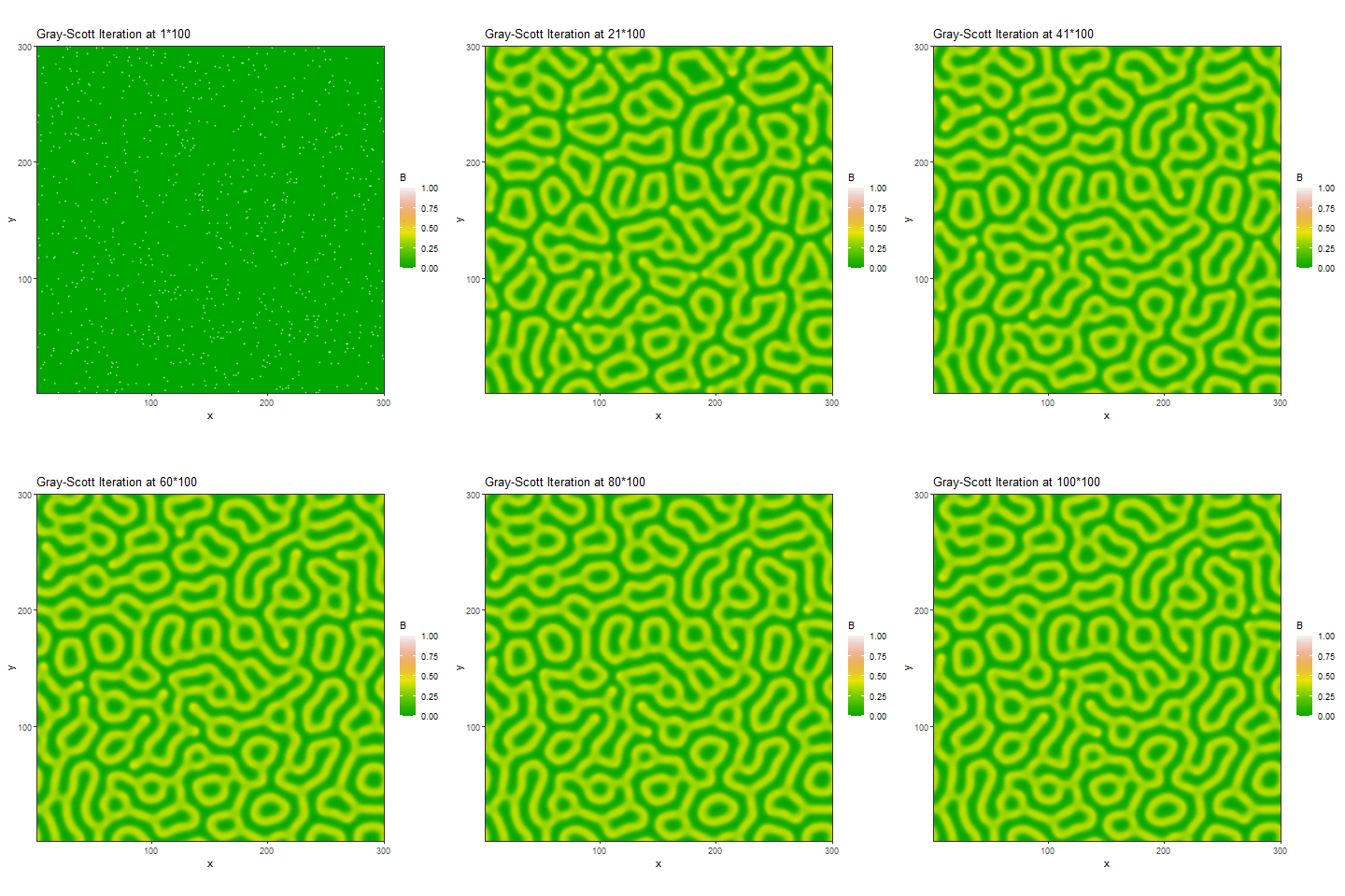

Note that the reaction diffusion model has two stable states: (1) Large \(A\) and no \(B\) to consume the \(A\) substance, and (2) Large \(B\) where any new \(A\) is quickly transformed into \(B\). However, the diffusion process can yield particular patterns at the borders between the two stable states. For instance, at convex borders, more \(A\) substance is available nearby to diffuse inwards and feed \(B\) causing edges to grow outwards as \(B\) increases and diffuses. On the other hand, at concave borders, less \(A\) diffuses in and \(B\) slowly shrinks, which causes \(B\) seeds to grow and divide, resembling the dynamics of cell mitosis.

The next simulation shows the reaction-diffusion dynamics for a varying kill rate, tracked over the horizontal \(x\) axis (\(0.045\leq k\leq 0.07\)), and a varying feed rate, along the vertical \(y\) axis (\(0.01\leq f\leq 0.1\)). The results show solid areas of pure substance \(A\) or substance \(B\), with a curvy-linear border zone in between showing complex mixture behavior of \(A\) and \(B\) components.

# Load in libraries
library(Rcpp)         # to iterate fast
library(tidyverse)    # to plot
library(reshape2)     # to melt matrix into data frame
library(colourlovers) # to color drawings with nice colors

# Import C++ code from https://socr.umich.edu/BPAD/support/
tf <- tempfile(fileext = ".cpp")
download.file("https://socr.umich.edu/BPAD/support/Gray_Scott_ReactionDiffusion_Cpp_funcs.cpp", tf, quiet=TRUE)
sourceCpp( tf )

# sourceCpp("E:/Ivo.dir/Research/BPAD/support/Gray_Scott_ReactionDiffusion_Cpp_funcs.cpp")

# Set ggplot aesthetics 
opt <-  theme(panel.border = element_rect(color="black", fill = NA),
              legend.position = "none",
              axis.ticks = element_blank(),
              panel.grid = element_blank(),
              axis.title = element_blank(),
              axis.text = element_blank())

# dimensions of plot outputs 300x300 pixels
pixels <- 300

# Initialize a pair of 2nd order tensors (matrices) A and B 
A <- matrix(1, pixels, pixels) # A is a fixed matrix of ones
B <- matrix(sample(c(0, 1),    # B is a binary matrix loaded for zeros 99:1
       size = pixels^2, replace = TRUE, prob = c(99,1)), ncol = pixels) 
# B <- matrix(0, pixels, pixels) 
# B[as.integer(pixels/2), as.integer(pixels/2)] <- 1

# 3*3 Convolution matrix L
L <- matrix(c(0.05, 0.2, 0.05, 
               0.2,  -1, 0.2, 
              0.05, 0.2, 0.05), nrow = 3)

# Try alternative settings
# e.g., DA=1.0, DB=0.5, f=0.055, k=0.062, Δt=1.0, or
#  f = 0.04, k = 0.06, DA = 0.01, DB = 0.005
# DA and DB parameters
DA <- 1.0
DB <- 0.5

# For fixed feed and kill rates
# f <- matrix(rep(0.0545, pixels), ncol = 1)
# k <- matrix(rep(0.062, pixels), ncol = 1)

f <- matrix(seq(from = 0.02, to = 0.08, length.out=pixels), ncol = 1)
k <- matrix(seq(from = 0.045, to = 0.07, length.out=pixels), ncol = 1)

# Create the tensor X
X <- array(c(A, B) , dim = c(pixels, pixels, 2))

# Run Gray-Scott algorithm iteratively - 10K iterations
iter_num <- 10000
X1 <- iterate_Gray_Scott_Dynamic(X, L, DA, DB, f, k, iter_num)

# Animation
library(ggplot2)
library(gganimate)

# Create an empty dataframe to hold all plot frames
plot_df <- data.frame(x = numeric(0), y = numeric(0),
                      B = numeric(0), GS_iteration = numeric(0))

# Compute all frames (taking every 100-th frame for speed)
for (i in 1:(iter_num/100)) {
  frame <- melt(X1[[(i-1)*100+1]][,,2])
  frame$GS_iteration <- i
  plot_df <- rbind(plot_df, frame)
}
# Rename columns ((x,y)-space, B-binary value, iteration-index)
colnames(plot_df) <- c("x","y","B", "GS_iteration") 

# render the animation
anim <- ggplot(plot_df, aes(x = x, y = y, fill= B)) +
  geom_raster(interpolate = T) +
  coord_equal() +
  scale_fill_gradientn(colours = terrain.colors(10)) +
  scale_y_continuous(expand = c(0,0)) + 
  scale_x_continuous(expand = c(0,0)) +
  opt +
  transition_manual(GS_iteration) +
  ggtitle("Gray-Scott Iteration using Varying f & k; iter={current_frame}*100") +
  coord_equal() +
  theme_bw()
# anim
anim_save("C:/Users/Dinov/Desktop/Gray_Scott_ReactionDiffusionAnimation_Dynamic_f_k.gif", anim)
knitr::include_graphics("https://socr.umich.edu/BPAD/support/Gray_Scott_ReactionDiffusionAnimation_Dynamic_f_k.gif")

Biomedical Physics with Applications to Disease (BPAD)

Chapter 5: Transport in Infinite Medium

BPAD Team + SOCR

January 2024

1 Reaction Diffusion